importNetworkFromPyTorch
Description
Add-On Required: This feature requires the Deep Learning Toolbox Converter for PyTorch Models add-on.
net = importNetworkFromPyTorch(modelfile)modelfile. The PyTorch model must be an exported program or a traced model. Exported program models
are recommended as they result in models with more Deep Learning Toolbox™ built-in layers.
Try exporting your model using PyTorch version 2.8 to prepare it for import. If the model cannot be exported, then trace it. See Tips for more information. The following code outlines the steps needed to prepare a PyTorch model for import:
# Ensure the layers are set to inference mode.
model.eval()
# Move the model to the CPU.
model.to("cpu")
# Generate input data.
X = torch.rand(1,3,224,224)

# For ExportedProgram models
# Export the model and save it in PyTorch version 2.8.
exported_model = torch.export.export(model, (X,))
torch.export.save(exported_model, 'myModel.pt2')

# For traced models
# Trace the model and save it.
traced_model = torch.jit.trace(model.forward, X)
traced_model.save('myModel.pt')
Alternatively, import PyTorch models interactively using the Deep Network Designer. On import, the app shows an import report with details about any issues that require attention. For more information, see Import Network from External Platform.
net = importNetworkFromPyTorch(modelfile,Name=Value)PyTorchInputSizes=[1 3 224 244]
may return more built-in Deep Learning Toolbox layers.
Examples
Import a PyTorch model trained on the CIFAR-10 [1] data. The model was saved in the exported program model format in PyTorch version 2.8 using the following Python code:
X = torch.rand(1,3,32,32)
exported_model = torch.export.export(model, (X,))
torch.export.save(exported_model, "exported_pytorch_model.pt2")
See Export and Save Trained PyTorch Model to learn more.
modelfile = "exported_pytorch_model.pt2";
net = importNetworkFromPyTorch(modelfile)
Importing the model, this may take a few minutes...
Warning: Some issues were found during translation, but no placeholders were generated:
Layer 'ResidualNetSmall:fc' has property OperationDimension set and requires its input to be in PyTorch dimension order.
net =
  dlnetwork with properties:

         Layers: [9×1 nnet.cnn.layer.Layer]
    Connections: [11×2 table]
     Learnables: [86×3 table]
          State: [42×3 table]
     InputNames: {'InputLayer1'}
    OutputNames: {'ResidualNetSmall:fc'}
    Initialized: 1

  View summary with summary.
If modifying the network after import, the software requires the input to the ResidualNetSmall:fc layer to be in the same order as was in the PyTorch network. For example, if the input to the linear layer in the original PyTorch network was 1-by-64, then the input to ResidualNetSmall:fc layer should also be 1-by-64.
Next, analyze the imported network layers.
analyzeNetwork(net)
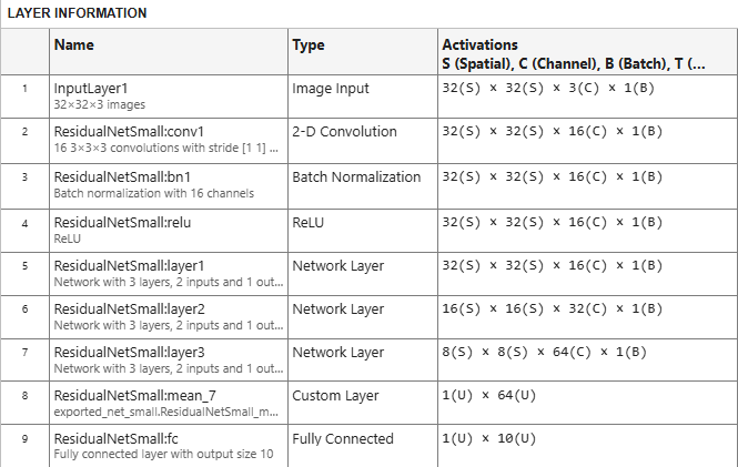
The imported network is composed of built-in MATLAB layers along with a custom layer.
[1] Krizhevsky, Alex. "Learning multiple layers of features from tiny images." (2009). https://www.cs.toronto.edu/~kriz/learning-features-2009-TR.pdf
Import a PyTorch model trained on the CIFAR-10 [1] data set. The model was saved in the exported program model format in PyTorch version 2.8.
See Export and Save Trained PyTorch Model to learn more.
modelfile = "exported_pytorch_model.pt2";
net = importNetworkFromPyTorch(modelfile)
The function imports the model as a dlnetwork object.
Download the CIFAR-10 data set. The data set contains 60,000 images. Each image is 32-by-32 pixels in size and has three color channels (RGB). The size of the data set is 175 MB. Depending on your internet connection, the download process can take time.
datadir = tempdir;
downloadCIFARData(datadir);
Load the CIFAR-10 test images as 4-D arrays. The test set contains 10,000 images. Use a CIFAR-10 test image for network validation.
[~,~,XValidation,TValidation] = loadCIFARData(datadir);
Display an image from the test data along with the label.
idx=1;
Im = XValidation(:,:,:,idx);
imshow(Im)
title("Label: "+string(TValidation(idx)))
Convert the image to a dlarray object. Format the image with the dimensions "SSCB" (spatial, spatial, channel, batch).
Im_dlarray = dlarray(single(Im),"SSCB");Classify the image and find the predicted label.
prob = predict(net,Im_dlarray);
predLabel = scores2label(prob,categories(TValidation));
disp("The predicted label is "+string(predLabel))
The predicted label is cat
[1] Krizhevsky, Alex. "Learning multiple layers of features from tiny images." (2009). https://www.cs.toronto.edu/~kriz/learning-features-2009-TR.pdf
Import a pretrained and traced PyTorch model as an initialized dlnetwork object using the name-value argument PyTorchInputSizes. See Trace and Save Trained PyTorch Model for detailed steps.
This example imports the MNASNet (Copyright© Soumith Chintala 2016) PyTorch model. MNASNet is an image classification model that is trained with images from the ImageNet database. Download the mnasnet1_0.pt file, which is approximately 17 MB in size, from the MathWorks website.
modelfile = matlab.internal.examples.downloadSupportFile("nnet", ...
    "data/PyTorchModels/mnasnet1_0.pt");
Import the MNASNet model by using the importNetworkFromPyTorch function with the name-value argument PyTorchInputSizes. We know that a 224x224 color image is a valid input size for this PyTorch model. The software automatically creates and adds the input layer for a batch of images. This allows the network to be imported as an initialized network in one line of code.
net = importNetworkFromPyTorch(modelfile,PyTorchInputSizes=[NaN,3,224,224])
Importing the model, this may take a few minutes...
Warning: Some issues were found during translation, but no placeholders were generated:
Layer 'MNASNet:classifier:1' has property OperationDimension set and requires its input to be in PyTorch dimension order.
net =
  dlnetwork with properties:

         Layers: [4×1 nnet.cnn.layer.Layer]
    Connections: [3×2 table]
     Learnables: [210×3 table]
          State: [104×3 table]
     InputNames: {'InputLayer1'}
    OutputNames: {'MNASNet:classifier'}
    Initialized: 1

  View summary with summary.
The network is ready to use for prediction.
Input Arguments
Name-Value Arguments
Output Arguments
Limitations
The
importNetworkFromPyTorchfunction supports exported networks created in PyTorch version 2.8. The function may be able to support traced networks created in other versions of PyTorch.Import of
ExportedProgramformat models exported with dynamic shapes is not supported.
More About
Tips
It is recommended to prepare PyTorch models for import by exporting them using
torch.export.export()over tracing. TheExportedProgramformat provides a stable, framework-independent file that captures the model’s computation graph, input and output specifications, and parameters in a deterministic structure. This format allows the software to import models that are initialized and comprising of more built-in MATLAB layers.Specify
PyTorchInputSizeswhen importing traced models to get better support for importing PyTorch layers into built-in MATLAB layers.To use a pretrained network for prediction or transfer learning on new images, you must preprocess your images in the same way as the images that you use to train the imported model. The most common preprocessing steps are resizing images, subtracting image average values, and converting the images from BGR format to RGB format.
For more information about preprocessing images for training and prediction, see Preprocess Images for Deep Learning.
The members of the
+namespace are not accessible if the namespace parent folder is not on the MATLAB path. For more information, see Namespaces and the MATLAB Path.NamespaceMATLAB uses one-based indexing, whereas Python uses zero-based indexing. In other words, the first element in an array has an index of 1 and 0 in MATLAB and Python, respectively. For more information about MATLAB indexing, see Array Indexing. In MATLAB, to use an array of indices (
ind) created in Python, convert the array toind+1.For more tips, see Tips on Importing Models from TensorFlow, PyTorch, and ONNX.
Algorithms
The importNetworkFromPyTorch function imports a PyTorch layer into MATLAB by trying these steps in order:
The function tries to import the PyTorch layer as a built-in MATLAB layer. For more information, see Conversion of PyTorch Layers.
The function tries to import the PyTorch layer as a built-in MATLAB function. For more information, see Conversion of PyTorch Layers.
The function tries to import the PyTorch layer as a custom layer.
importNetworkFromPyTorchsaves the generated custom layers and the associated functions in the+namespace.NamespaceThe function imports the PyTorch layer as a custom layer with a placeholder function. You must complete the placeholder function before you can use the network, see Placeholder Functions.
In the first three cases, the imported network is ready for prediction after you initialize it.
Alternative Functionality
App
You can also import networks from external platforms by using the Deep Network Designer app. The app uses the
importNetworkFromPyTorch function to import the network, and displays a progress
dialog box. During the import process, the app adds an input layer to the network, if
possible, and displays an import report with details about any issues that require
attention. After importing a network, you can interactively edit, visualize, and analyze the
network. When you are finished editing the network, you can export it to Simulink® or generate MATLAB code for building networks.
Block
You can also work with PyTorch networks by using the PyTorch Model Predict block. This block additionally allows you to load Python functions to preprocess and postprocess data, and to configure input and output ports interactively.