Posterior Estimation and Simulation Diagnostics

Empirical, custom, and semiconjugate prior models yield analytically intractable posterior distributions (for more details, see Analytically Intractable Posteriors). To summarize the posterior distribution for estimation and inference, the first model requires Monte Carlo sampling, while the latter two models require Markov Chain Monte Carlo (MCMC) sampling. When estimating posteriors using a Monte Carlo sample, particularly an MCMC sample, you can run into problems resulting in samples that inadequately represent or do not summarize the posterior distribution. In this case, estimates and inferences based on the posterior draws can be incorrect.

Even if the posterior is analytically tractable or your MCMC sample represents the true posterior well, your choice of a prior distribution can influence the posterior distribution in undesirable ways. For example, a small change to the prior distribution, such as a small increase in the value of a prior hyperparameter, can have a large effect on posterior estimates or inferences. If the posterior is that sensitive to prior assumptions, then interpretations of statistics and inferences based on the posterior might be misleading.

Therefore, after obtaining the posterior distribution from a sampling algorithm, it is important to determine the quality of the sample. Also, regardless of whether the posterior is analytically tractable, it is important to check how sensitive the posterior is to prior distribution assumptions.

Diagnose MCMC Samples

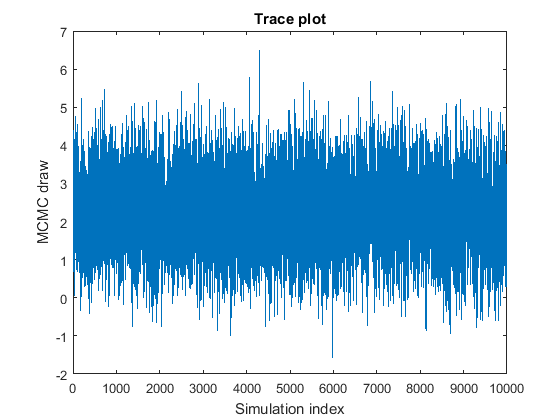
When drawing an MCMC sample, a good practice is to draw a smaller, pilot sample, and then view trace plots of the drawn parameter values to check whether the sample is adequate. Trace plots are plots of the drawn parameter values with respect to simulation index. A satisfactory MCMC sample reaches the stationary distribution quickly and mixes well, that is, explores the distribution in broad steps with little to no memory of the previous draw. This figure is an example of a satisfactory MCMC sample.

This list describes problematic characteristics of MCMC samples, gives an example of what to look for in the trace plot, and describes how to address the problem.

• The MCMC sample appears to travel to the stationary distribution, that is, it displays transient behavior.

  

  To remedy the problem, use one of the following techniques:

  • Specify starting values for the parameters that are closer to the mean of the stationary distribution, or specify a value that you expect in the posterior, using the BetaStart and Sigma2Start name-value pair arguments.

  • Specify a burn-in period, that is, the number draws starting from the beginning to remove from the posterior estimation, using the BurnIn name-value pair argument. The burn-in period should be large enough so that the remaining sample resembles a satisfactory MCMC sample, and small enough so that the adjusted sample size is sufficiently large.

• The MCMC sample displays high serial correlation. The following figures are the trace plots and autocorrelation function (ACF) plots (see autocorr).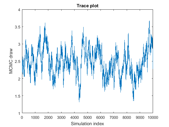

  

  

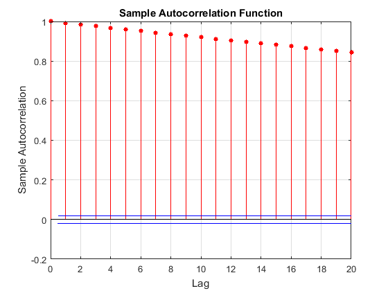
  The trace plot shows that subsequent samples seem to be a function of past samples. The ACF plot is indicative of a process with high autocorrelation.

  Such MCMC samples mix poorly and take a long time to sufficiently explore the distribution. Try the following:

  • If you have enough resources, then estimates based on large MCMC samples are approximately correct.

  • To reduce high autocorrelation, you can retain a fraction of the MCMC sample by thinning using the Thin name-value pair argument.

  • For custom prior models, try a different sampler by using the 'Sampler' name-value pair argument. To adjust tuning parameters of the sampler, create a sampler options structure instead by using sampleroptions, which allows you to specify a sampler and values for its tuning parameters. Then, pass the sampler options structure to estimate, simulate, or forecast by using the 'Options' name-value pair argument.

• The MCMC sample jumps from state to state.

  

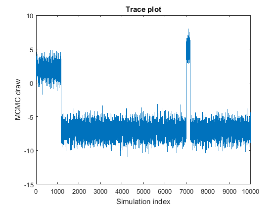
  The plot shows subsamples centered at the values 2, –7, and 5, which mix well. This behavior might indicate one of the following qualities:

  • At least one of the parameters is not identifiable. You might have to reform your model and assumptions.

  • There might be coding issues with your Gibbs sampler.

  • The stationary distribution is multimodal. In this example, the probability of being in the state centered at –7 is highest, followed by 2, and then 5. The probability of moving out of the state centered at 7 is low.

    If your prior is strong and your sample size is small, then you might see this type of MCMC sample, which is not necessarily problematic.

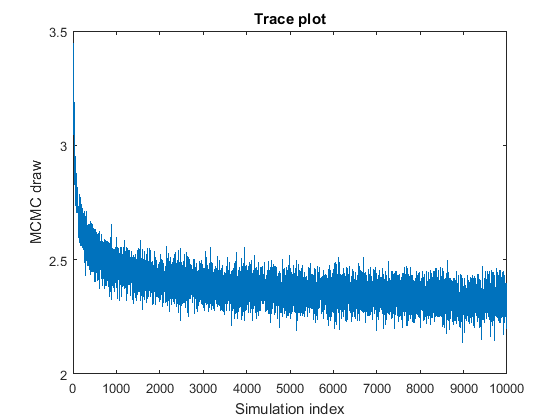
• The Markov chain does not converge to its stationary distribution.

  

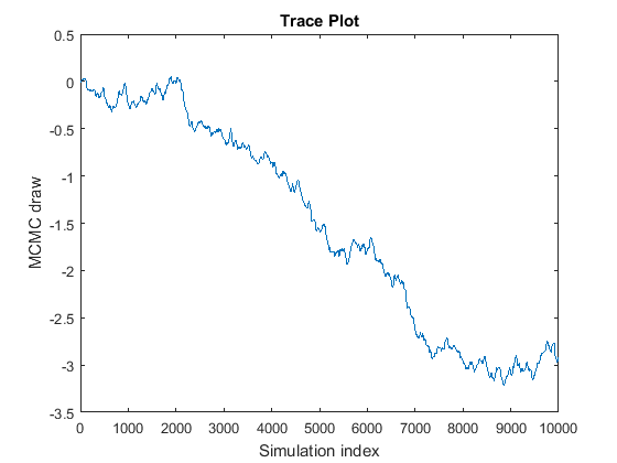
  The curve looks like a random walk because the MCMC is slowly exploring the posterior. If this problem occurs, then posterior estimates based on the MCMC sample are incorrect. To remedy the problem, try the following techniques:

  • If you have enough resources, draw many more samples, and then determine whether the chain eventually settles and marginally mixes. If it does settle and mix relatively well, then remove the beginning portion of the sample, and consider thinning the rest of the sample. For example, suppose that you draw 20000 samples of the chain in the figure, and then you find that the chain settles around -3 after 7000 draws. You can treat draws 1:7000 as burn-in (BurnIn), and then thin (Thin) the remaining draws to achieve a satisfactory level of autocorrelation.

  • Reparameterize the prior distribution. When estimating customblm model objects, you can specify reparameterization of the disturbance variance to the log scale using the Reparameterize name-value pair argument.

  • For custom prior models, try a different sampler by using the 'Sampler' name-value pair argument. To adjust tuning parameters of the sampler, create a sampler options structure instead by using sampleroptions, which allows you to specify a sampler and values for its tuning parameters. Then, pass the sampler options structure to estimate, simulate, or forecast by using the 'Options' name-value pair argument.

In addition to trace and ACF plots, estimate, simulate, and forecast estimate the effective sample size. If the effective sample size is less than 1% of the number of observations, then those functions throw warnings. For more details, see [1].

Perform Sensitivity Analysis

A sensitivity analysis includes determining how robust posterior estimates are to prior and data distribution assumptions. That is, the goal is to learn how replacing initial values and prior assumptions with reasonable alternatives affects the posterior distribution and inferences. If the posterior and inferences do not vary much with respect to the application, then the posterior is robust to prior assumptions and initial values. Posteriors and inferences that do vary substantially with varying initial assumptions can lead to incorrect interpretations.

To perform a sensitivity analysis:

1. Identify a set of reasonable prior models. Include diffuse (diffuseblm) models and subjective (conjugateblm or semiconjugateblm) models that are easier to interpret and allow inclusion of prior information.

2. For each of the prior models, determine a set of plausible hyperparameter values. For example, for normal-inverse-gamma conjugate or semiconjugate prior models, choose various values for the prior mean and covariance matrix of the regression coefficients and the shape and scale parameters of the inverse gamma distribution of the disturbance variance. For more details, see the Mu, V, A, and B name-value pair arguments of bayeslm.

3. For all prior model assumptions:

   1. Estimate corresponding posteriors using estimate.

   2. Draw inferences using the posterior. For example, obtain 95% equitailed credible intervals or forecast responses given predictor data using forecast.

4. Compare the estimates and inferences among the models.

   • If all estimates and inferences are similar enough, then the posterior is robust.

   • If estimates or inferences are sufficiently different, then there might be some underlying problem with the selected priors or data likelihood. Because the Bayesian linear regression framework in Econometrics Toolbox™ always assumes that the data are Gaussian, consider:

     • Adding or removing predictor variables from the regression model

     • Making the priors more informative

     • Completely different prior assumptions

For more details on sensitivity analysis, see [2], Ch. 6.

References

[1] Geyer, C. J. “Practical Markov chain Monte Carlo.” Statistical Science. Vol. 7, 1992, pp. 473-483.

[2] Gelman, A., J. B. Carlin, H. S. Stern, and D. B. Rubin. Bayesian Data Analysis, 2nd. Ed. Boca Raton, FL: Chapman & Hall/CRC, 2004.