Initialize Incremental Learning Model from Logistic Regression Model Trained in Classification Learner

This example shows how to train a logistic regression model using the Classification Learner app. Then, at the command line, initialize and train an incremental model for binary classification using the information gained from training in the app.

Load and Preprocess Data

Load the human activity data set. Randomly shuffle the data.

load humanactivity
rng(1); % For reproducibility
n = numel(actid);
idx = randsample(n,n);
X = feat(idx,:);
actid = actid(idx);

For details on the data set, enter Description at the command line.

Responses can be one of five classes: Sitting, Standing, Walking, Running, or Dancing. Dichotomize the response by creating a categorical array that identifies whether the subject is moving (actid > 2).

moveidx = actid > 2;
Y = repmat("NotMoving",n,1);
Y(moveidx) = "Moving";
Y = categorical(Y);

Consider training a logistic regression model to about 1% of the data, and reserving the remaining data for incremental learning.

Randomly partition the data into 1% and 99% subsets by calling cvpartition and specifying a holdout (test) sample proportion of 0.99. Create variables for the 1% and 99% partitions.

cvp = cvpartition(n,'HoldOut',0.99);
idxtt = cvp.training;
idxil = cvp.test;

Xtt = X(idxtt,:);
Xil = X(idxil,:);
Ytt = Y(idxtt);
Yil = Y(idxil);

Train Model Using Classification Learner

Open Classification Learner by entering classificationLearner at the command line.

classificationLearner

Alternatively, on the Apps tab, click the Show more arrow to open the apps gallery. Under Machine Learning and Deep Learning, click the app icon.

Choose the training data set and variables.

1. On the Classification Learner tab, in the File section, select New Session > From Workspace.

2. In the New Session from Workspace dialog box, under Data Set Variable, select the predictor variable Xtt.

3. Under Response, click From workspace; note that Ytt is selected automatically.

4. Under Validation Scheme, select Resubstitution Validation.

5. Click Start Session.

Train a logistic regression model.

1. On the Classification Learner tab, in the Models section, click the Show more arrow to open the gallery of models. In the Logistic Regression Classifiers section, click Logistic Regression.

2. On the Classification Learner tab, in the Train section, click Train All and select Train Selected.

   After training the model, the app displays a confusion matrix.

   

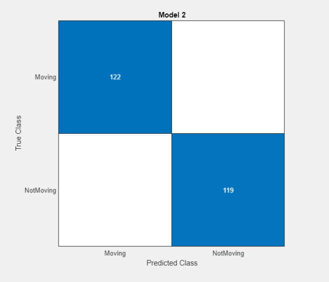
   The confusion matrix suggests that the model classifies in-sample observations well.

Export the trained logistic regression model.

1. On the Classification Learner tab, in the Export section, select Export Model > Export Model.

2. In the Export Model dialog box, click OK.

The app passes the trained model, among other variables, in the structure array trainedModel to the workspace. Close Classification Learner .

Initialize Incremental Model Using Exported Model

At the command line, extract the trained logistic regression model and the class names from trainedModel. The model is a GeneralizedLinearModel object. Because class names must match the data type of the response variable, convert the stored value to categorical.

Mdl = trainedModel.GeneralizedLinearModel;
ClassNames = categorical(trainedModel.ClassNames);

Extract the intercept and the coefficients from the model. The intercept is the first coefficient.

Bias = Mdl.Coefficients.Estimate(1);
Beta = Mdl.Coefficients.Estimate(2:end);

You cannot convert a GeneralizedLinearModel object to an incremental model directly. However, you can initialize an incremental model for binary classification by passing information learned from the app, such as estimated coefficients and class names.

Create an incremental model for binary classification directly. Specify the learner, intercept, coefficient estimates, and class names learned from Classification Learner. Because good initial values of coefficients exist and all class names are known, specify a metrics warm-up period of length 0.

IncrementalMdl = incrementalClassificationLinear('Learner','logistic', ...
    'Beta',Beta,'Bias',Bias,'ClassNames',ClassNames, ...
    'MetricsWarmupPeriod',0)

IncrementalMdl = 

  incrementalClassificationLinear

            IsWarm: 0
           Metrics: [1×2 table]
        ClassNames: [Moving    NotMoving]
    ScoreTransform: 'logit'
              Beta: [60×1 double]
              Bias: -471.7873
           Learner: 'logistic'


  Properties, Methods

IncrementalMdl is an incrementalClassificationLinear model object for incremental learning using a logistic regression model. Because coefficients and all class names are specified, you can predict responses by passing IncrementalMdl and data to predict.

Implement Incremental Learning

Perform incremental learning on the 99% data partition by using the updateMetricsAndFit function. Simulate a data stream by processing 50 observations at a time. At each iteration:

1. Call updateMetricsAndFit to update the cumulative and window classification error of the model given the incoming chunk of observations. Overwrite the previous incremental model to update the losses in the Metrics property.

2. Store the losses and the estimated coefficient β₁₄.

% Preallocation
nil = sum(idxil);
numObsPerChunk = 50;
nchunk = floor(nil/numObsPerChunk);
ce = array2table(zeros(nchunk,2),'VariableNames',["Cumulative" "Window"]);
beta14 = [IncrementalMdl.Beta(14); zeros(nchunk,1)];

% Incremental learning
for j = 1:nchunk
    ibegin = min(nil,numObsPerChunk*(j-1) + 1);
    iend   = min(nil,numObsPerChunk*j);
    idx = ibegin:iend;
    IncrementalMdl = updateMetricsAndFit(IncrementalMdl,Xil(idx,:),Yil(idx));
    ce{j,:} = IncrementalMdl.Metrics{"ClassificationError",:};
    beta14(j + 1) = IncrementalMdl.Beta(14);
end

IncrementalMdl is an incrementalClassificationLinear model object trained on all the data in the stream.

Plot a trace plot of the performance metrics and β₁₄.

figure;
subplot(2,1,1)
h = plot(ce.Variables);
xlim([0 nchunk]);
ylabel('Classification Error')
legend(h,ce.Properties.VariableNames)
subplot(2,1,2)
plot(beta14)
ylabel('\beta_{14}')
xlim([0 nchunk]);
xlabel('Iteration')

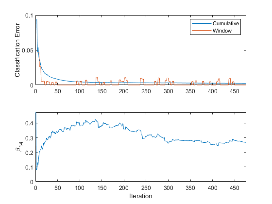
The cumulative loss gradually changes with each iteration (chunk of 50 observations), whereas the window loss jumps. Because the metrics window is 200 by default and updateMetricsAndFit measures the performance every four iterations.

β₁₄ adapts to the data as updateMetricsAndFit processes chunks of observations.