Results for
I spent some time tonight updating the UIHTML App skills on the MATLAB Agent Skills Playground hosted on GitHub.
We are using this repo to share early ideas and experiments with agent skills.
When you are trying to bring the latest update into a coding like Codex, you can point the agent at a secret file called "llms.txt" -- this is file optimized for coding agents. I use it to over come "training data" bias. As even the latest models have outdated doc. This is important for working with projects that up date frequently.
Here are some of my favorites to use:
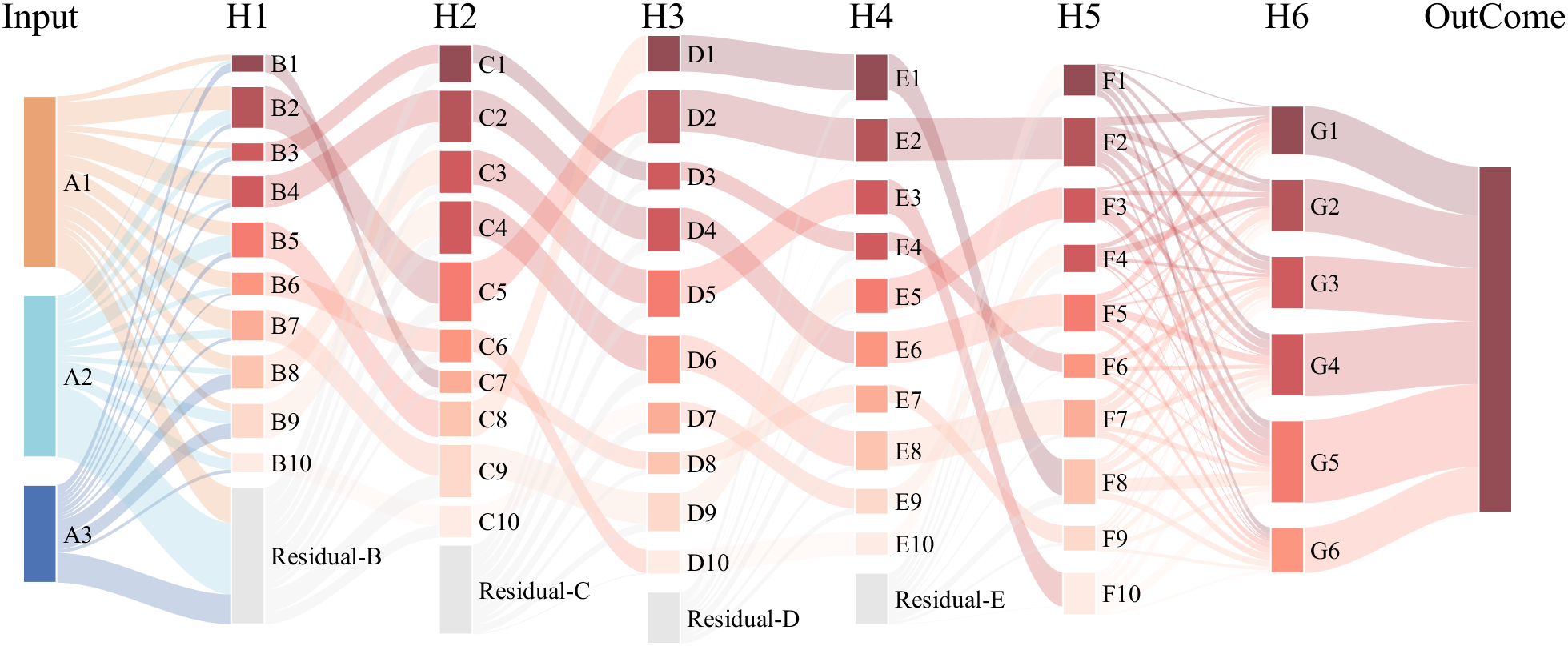
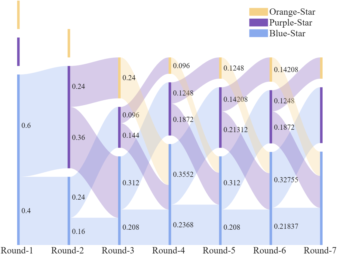
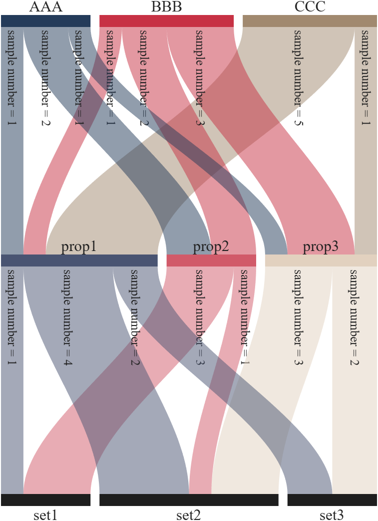
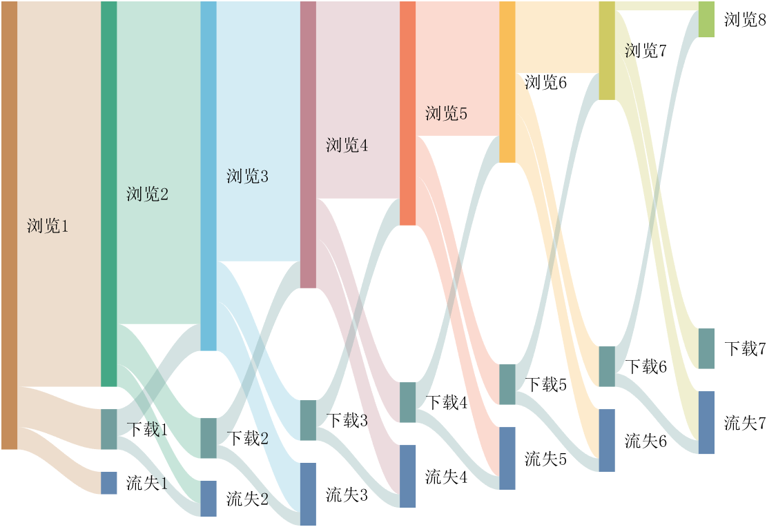
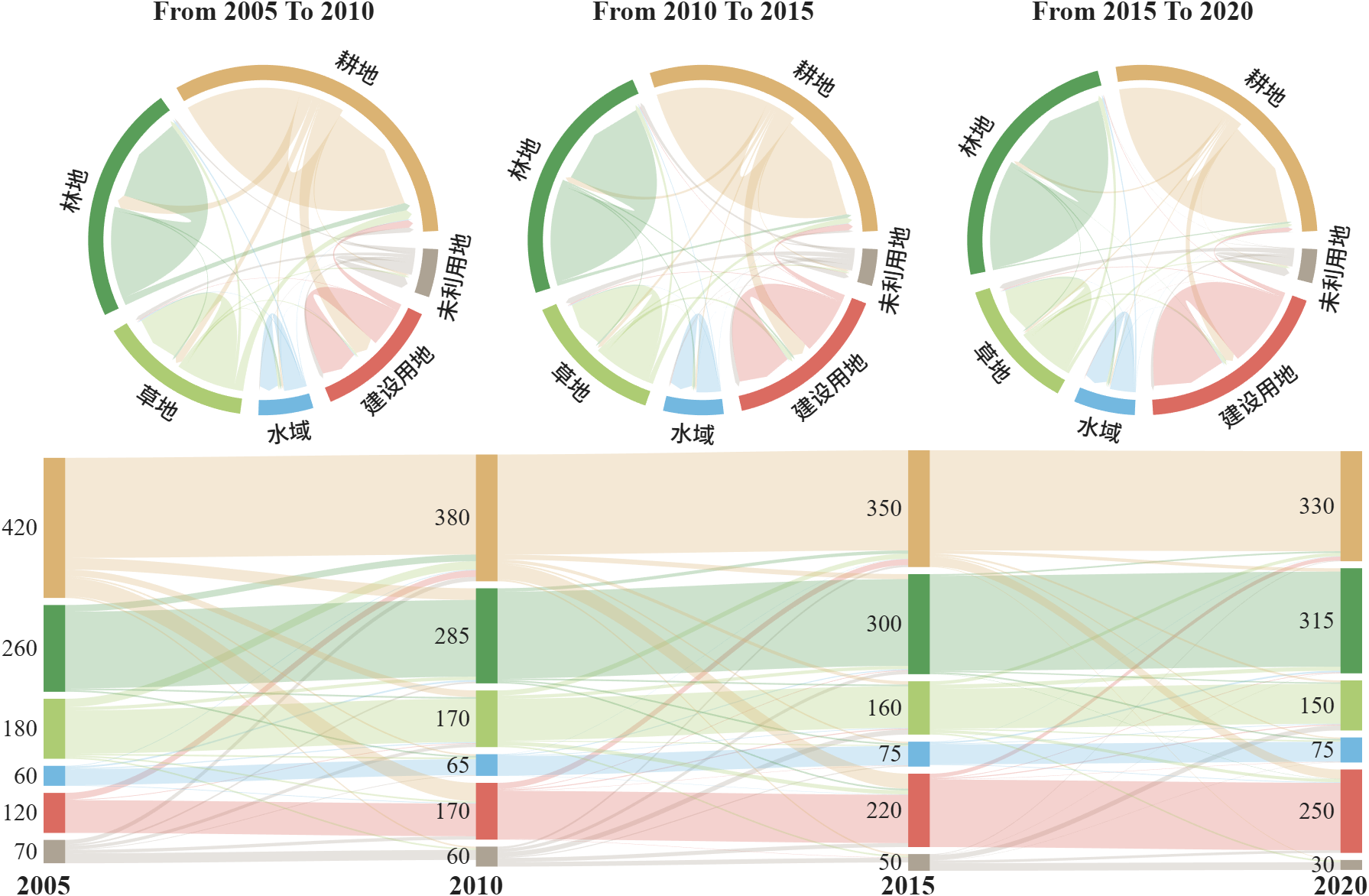
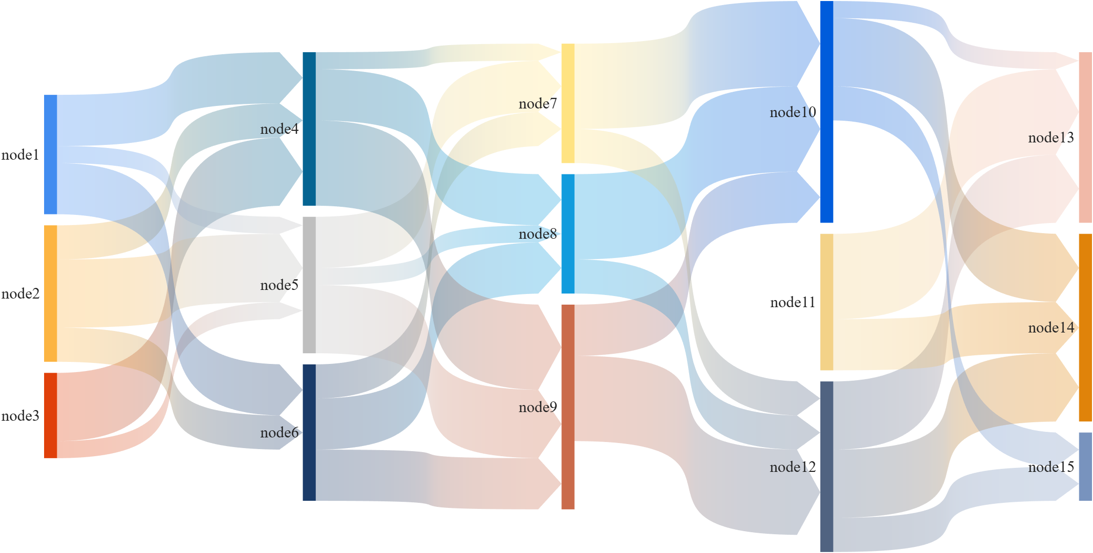
This is a brief introduction and recommendation of a Sankey diagram plotting tool:
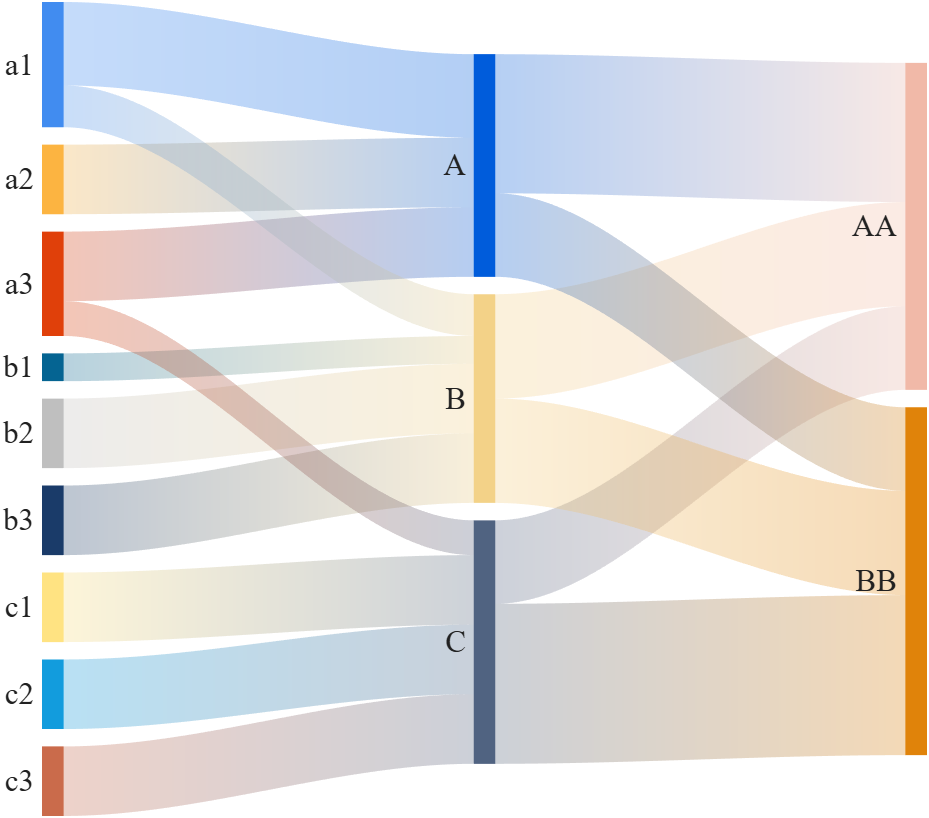
Basic usage - links
links={'a1','A',1.2;'a2','A',1;'a1','B',.6;'a3','A',1; 'a3','C',0.5;
'b1','B',.4; 'b2','B',1;'b3','B',1; 'c1','C',1;
'c2','C',1; 'c3','C',1;'A','AA',2; 'A','BB',1.2;
'B','BB',1.5; 'B','AA',1.5; 'C','BB',2.3; 'C','AA',1.2};
% 创建桑基图对象(Create a Sankey diagram object)
SK=SSankey(links(:,1),links(:,2),links(:,3));
% 开始绘图(Start drawing)
SK.draw()
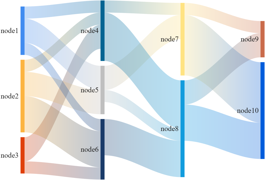
Basic usage - adjMat
% Define inter-layer adjacency matrices
% 定义层间邻接矩阵
A12 = [1,2,1; 1,2,3; 2,0,1];
A23 = [1,4; 2,1; 0,3];
A34 = [1,5; 2,3];
% Assemble global block matrix (main diagonal = zero, super-diagonal = A12, A23, A34)
% 组装全局分块矩阵(主对角线为零,上对角线为 A12, A23, A34)
adjMat = mergeAdjMat({A12, A23, A34});
SK = SSankey([],[],[], 'AdjMat',adjMat);
SK.draw()
Further usage examples can be found in the demos included in the compressed package:
MATLAB Editor (built-in editor)
77%
VS Code (Visual Studio Code)
20%
Jupyter Notebook / MATLAB Kernel
2%
PyCharm (via plugins or external )
1%
Sublime Text / Atom
0%
Others (please specify in commets)
0%
191 votes
Hello everyone,
Does anyone know of a reliable tool (or workflow) that can automatically convert MATLAB code to C++ code? I am aware of MATLAB Coder, but I would like to know if there are any third‑party tools or scripts that can perform a similar translation, especially for numerical/computational code.
Any suggestions or experiences would be greatly appreciated. Thank you!
I follow a lot of astronomical/astrophysical missions and notice they have now gotten massive in size, scope, and data. Petabyte datasets are now commonplace. Some are now moving essentially to private clouds where researchers create accounts and use primarily FOSS tools to process data. Some examples are the Vera Rubin Observatory's Rubin Science Platform and ESA's Datalabs. Jupyter has entrenched itself deeply despite its many shortcomings. I can't create accounts on any of these platforms but I am guessing that getting support for license-servers and other paraphernalia associated with closed-source software won't be easy.
It makes sense at some level when datasets get so big they can't be practically served to a researcher's machine. But, I do wonder what this public data in private clouds means for MATLAB and similar paid software. All the projects say that FOSS encourages reproducibility but I've been burned more than once in my working life by randomly phased Python package updates and abandoned projects.
I'm retired now and don't have a dog in the fight. My MATLAB home license is just for self-improvement. I was just curious whether Mathworks and similar providers will have to give up on the basic science community and focus on applied, mission-critical areas where "some guy on Github" is not sufficient traceability.
Hi everyone,
I'm interested in learning how developers compare code, configuration files, JSON data, or text changes when working outside of version control systems.
Common scenarios include:
- Comparing two versions of a script
- Reviewing generated output
- Checking configuration changes
- Comparing API responses or JSON files
- Reviewing documentation updates
I've used IDE comparison features and online diff tools. One browser-based tool I've found useful for quick comparisons is Text Differ:
I'm curious what workflows or tools other community members prefer. Do you rely on built-in editor features, version control diffs, or dedicated comparison tools?
Looking forward to hearing your experiences.
MATLAB AI Agent SDK lets you build and run AI agents in MATLAB.
- Create agents based on OpenAI®, Ollama™, or OpenAI-compatible APIs.
- Integrate LLMs and agentic workflows into your workflows in a targeted manner, retaining deterministic workflows when those are more suitable.
- Let your agent work on large amounts of data without needing to send the data to the LLM.
This SDK is a Research Preview under active development and APIs may change.
How much faster does a small GPT train on an Apple Silicon GPU?
Duncan Carlsmith, Department of Physics, University of Wisconsin-Madison
Introduction
My prior post nanoGPT Arithmetic Explorer: A small MATLAB GPT that groks integer addition, and my FEX submission nanoGPT Arithmetic Explorer present a small character-level GPT in MATLAB that learns integer addition, trained entirely on the CPU. That project raised for me a practical question for anyone who, like me, runs MATLAB on a Mac: MATLAB has no GPU support on Apple Silicon - gpuArray and the Deep Learning Toolbox training path require an NVIDIA CUDA GPU - yet every M-series Mac carries a capable GPU, arguably a built-in NVIDIA Spark equivalent, that sits idle while the model trains. APPLE GPUs have reduced precision, but that is perhaps not relevant, even valued, in GPT applications. To access the APPLE GPU requires indirect methods. My new Live Script Mac GPT GPU Benchmark Explorer explores the speed up for small models with a small, reproducible GPT benchmark for any Mac.
The workload is the same small GPT learning addition, so each variant can be checked to actually learn - to grok perfect answers on held-out problems. The same model is trained three ways on the same machine: the original MATLAB engine on the CPU, PyTorch on the CPU, and PyTorch on the Metal GPU through Apple's MPS backend. Three points let the total speedup factor into a framework effect and a device effect. The nanoGPT model is flexible in size, allowing extrapolation to larger models not needed in the arithmetic application.
On my M1 Max, the result is about a 7.7x speedup per training step moving from the MATLAB workflow to PyTorch on the GPU, and it factors as roughly 3.7x from the framework times 2.1x from the device. Most of the gain is not the GPU: likely PyTorch's fused attention, tuned linear algebra, and lighter automatic differentiation account for the larger factor, and the Metal GPU roughly doubles it again. With a fixed model seed, the CPU and GPU loss curves agree to several decimals, and both grok to perfect accuracy, so this is the same computation, only faster - all in single precision, which is what neural-network training often uses anyway and what every Apple GPU provides.
The script also pits Apple's own MLX framework against PyTorch on the GPU. MLX has its own Metal kernels and edges, PyTorch only for the smallest models; PyTorch pulls ahead as the model grows. A size sweep shows the GPU advantage ranging from roughly two to six times across a wide range of model sizes. Caveats: a laptop throttles under sustained load, so a long run reads slower per step than a short, timed burst. Other factors may enter. I'm no expert in benchmarking practices.
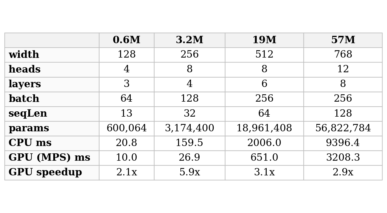
Table 1. The size sweep on the reference machine (Apple M1 Max): each column is one model configuration, headed by its parameter count, with the per-step training time on the CPU and on the Apple GPU (PyTorch-MPS). GPU speedup is CPU time divided by GPU time. It is a compound sweep - width, heads, layers, batch, and sequence length all change together.
 The Live Script is organized as three panels - the three-point comparison, the speedup-versus-size sweep, and the MLX-versus-PyTorch contrast. Each panel displays a precomputed result shipped with the package by default, and each has a "Try this" switch that regenerates it on your own Mac. A set of challenges suggests the reader extend the study, for example, with controlled single-variable sweeps or a run on a different Apple chip. The self-contained arithGPT trainer is bundled with the script; the GPU work runs in PyTorch and MLX, both free and open-source, with no paid API. The package and this writeup were built with Claude (Anthropic) working with MATLAB R2026a on my own MacBook with an M1 chip through an ngrok command server, the agentic context described in my prior posts.
A note on hardware: what "capable" means
Three numbers describe a GPU for this kind of work. Compute is measured in TFLOPS - trillions of floating-point arithmetic operations per second - quoted at a stated numeric precision; FP32 means 32-bit floating-point numbers, the full-precision arithmetic this article trains in, and the standard for scientific computing. Memory bandwidth, in gigabytes per second (GB/s), is how fast the chip moves data between memory and its arithmetic units; for the small models trained here, that is often the real limit, rather than raw compute. Unified memory, in gigabytes (GB), is the single pool of memory that the CPU and GPU share on these chips, which sets how large a model can be held at once. The last row of the table is simply whether MATLAB's own GPU functions (gpuArray, trainnet) run on the machine: they require NVIDIA's CUDA platform, which no Apple Silicon Mac provides.
Table 2. GPU capability of the M1 Max used in this study, Apple's current M5 and M5 Max, and NVIDIA's DGX Spark, all at FP32 precision. Higher TFLOPS and bandwidth are faster; unified memory sets the largest model that fits; the last row is whether MATLAB's built-in GPU training runs on the machine.
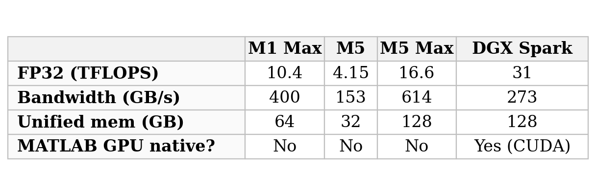
The M1 Max used here delivers about 10 TFLOPS of FP32 at 400 GB/s - genuinely capable, and in fact more memory bandwidth than the brand-new DGX Spark. Apple's current line runs from the small M5 (4.15 TFLOPS, lower than the older M1 Max because it is the entry-level chip) up to the M5 Max (16.6 TFLOPS, 614 GB/s, 128 GB), the true successor that beats the M1 Max on every count.
The DGX Spark plays a different game. Its FP32 figure of about 31 TFLOPS is only part of the story; its real strength is arithmetic at very low precision, which Apple's GPUs do not offer. NVIDIA's headline 'one petaFLOP' (a thousand TFLOPS) is an FP4 number - 4-bit floating-point, sixteen times coarser than FP32 - and it also counts sparsity, a hardware trick that skips multiplications by zero; without that trick, it is about half as much. Four-bit numbers are far too coarse to train with, but they are precise enough to run an already-trained very large model, which is what the Spark is built for: large-model use on the desktop, not the full-precision training measured here. The detail that matters for this article is the last table row - because the Spark runs CUDA on Linux, MATLAB's own GPU training path works on it directly, the very thing that does not exist on any Mac, and the reason this study reached for PyTorch and MLX.
References
Duncan Carlsmith (2026). Mac GPT GPU Benchmark Explorer (https://www.mathworks.com/matlabcentral/fileexchange/184058-mac-gpt-gpu-benchmark-explorer), MATLAB Central File Exchange. Retrieved June 12, 2026.
Acknowledgements
This submission and the FEX submission build and test were made with the assistance of Anthropic Claude in a few hours. The author has relied heavily on Claude's expertise. Caveat emptor.
Conflict of interest
The author declares he has no financial interest in MathWorks, Anthropic, or Apple. This article is informational and does not constitute an endorsement by the University of Wisconsin-Madison of any vendor or product. Claude is a trademark of Anthropic. MATLAB is a trademark of MathWorks. PyTorch, MLX, and Metal are trademarks of their respective owners.
We’re excited to share that our new unified search experience is now live!
Anywhere you see the MATLAB Help Center | Community | Learning header, the search icon will now take you to the same results page. This makes it much easier to find content across different areas in one place—and you’ll also see an AI-powered response at the top to help you get quick answers.
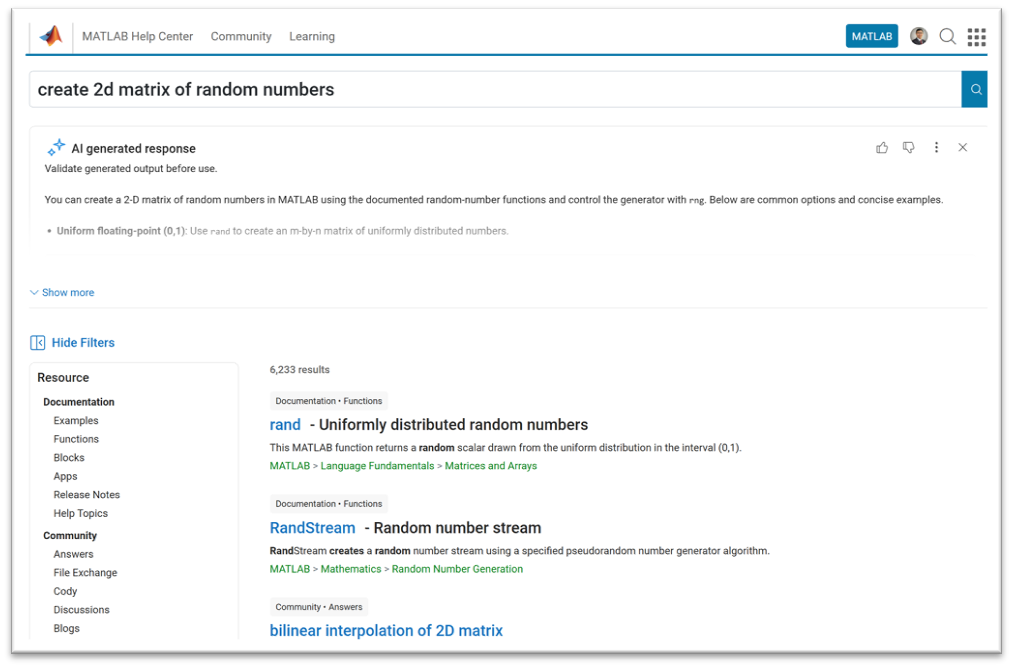
A quick note: search from the homepage, product pages, solutions, and a few other areas will continue to work as they do today.
This update is all about making it easier to discover related content across the site, instead of being limited to one area at a time.
Give it a try and let us know what you think—we’d love your feedback!
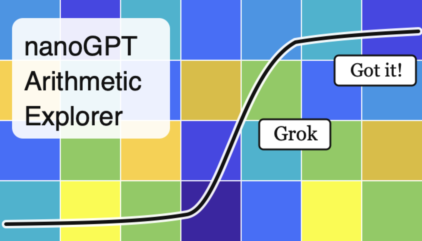 A small MATLAB GPT that groks integer addition
Duncan Carlsmith, Department of Physics, University of Wisconsin-Madison
Introduction
My prior post A miniature GPT language model as a MATLAB Live Script provides a small character-level GPT in MATLAB and trains it on Shakespeare. Language modeling is intractable in the sense that there is no exact answer to grade against; the model is judged by whether its output reads plausibly. This companion Live Script applies the same architecture to a problem with a clear success metric. The goal of training is for the model to discover/get/“grok” an exact algorithm for integer addition in any base (e.g., binary, decimal, and hexadecimal). With this script, you can watch a “grok,” the model suddenly “getting” addition, happen in real time and in detail- very fun if you are like me, hardly an expert!
Addition is easy except for the carry. The digit in a column is the column sum modulo the base. The carry couples columns: a carry out of one column feeds the next, and consecutive carries chain groups of columns together. The script grades the model on held-out problems sorted by the length of the longest carry chain, so the per-chain accuracy curves show exactly where and how the model succeeds. One observes the model first grok single carries, then singles and doubles, and so on, up to the maximum for the range of digits presented during training. In representing a finite range of numbers, the distribution of carry chain lengths depends on the base, as does the number of essential tokens. Hence, although the essence of addition is base-independent, the learning curves are different for different bases.
As is well known, the grok duration can be very short or gradual, depending on exactly how the addition problem is posed when presented to the model and if a random or structured learning curriculum is used. The script demonstrates that since a random number generator based on a seed is used to generate training samples, the time and even existence of a grok in a prescribed length set of training steps fluctuates, sometimes wildly, but for the same seed, and training is reproducible deterministically to machine precision. Comparative studies of the efficacy of different model sizes, problem presentation formats, and training curricula require statistical analysis and are not attempted by this script.
The Live Script is organized as five experiments. The first trains naively on random problems and can show a vexing carry stall - a partial grok. The next two use a difficulty curriculum that orders training from short carry chains to long ones, and a scratchpad format that writes each column's digit and carry explicitly so the carry is a token in context rather than something inferred. The fourth combines both. The fifth trains one model on a mix of bases, each problem labeled with its base, and tests a base never seen in training; the base-independent column sum transfers to the new base, but the base-specific carry threshold does not. Each experiment displays a precomputed figure by default. Each also has a "Try this" switch that retrains it live with your own base, digit count, model size, and seed. A set of challenges asks the reader to extend the work, for example, to test length generalization or study subtraction together with addition.
The engine that does the training and evaluation is a set of MATLAB functions shipped with the script and usable on their own from the Command Window, independent of the Live Script. An accompanying guide documents them for readers who want to understand the details or run their own experiments. The script and engine were built with Claude (Anthropic) working with MATLAB R2026a on my own MacBook with an M1 chip through an ngrok command server, the agentic context described in my prior posts. No GPU or API is used.
References
Duncan Carlsmith (2026). nanoGPT Arithmetic Explorer (https://www.mathworks.com/matlabcentral/fileexchange/184054-nanogpt-arithmetic-explorer), MATLAB Central File Exchange. Retrieved June 11, 2026.
Conflict of interest
The author declares he has no financial interest in MathWorks or Anthropic. This article is informational and does not constitute an endorsement by the University of Wisconsin-Madison of any vendor or product. Claude is a trademark of Anthropic. MATLAB is a trademark of MathWorks.
I've been confused trying to write (or have an AI write) the .m (Live) text format from scratch for various reasons using .mlx format exported with the IDE as .m (old) and .m (LIve). Of course, one problem is the .m and .m (Live) files have the same name,causing confusion and requiring renaming, but repeatedly, after sussing out and following all conventions for headings and latex etc in .m (LIve), my .m (Live) files would not open as .mlx in the IDE. I think I've found the answer by trial and error and comparison and don't know it is documented. Add at the end
%[appendix]{"version":"1.0"} %--- %[metadata:view] % data: {"layout":"inline"} %---
This seems to trigger the IDE to recognize this is a .m (Live). Woohoo! This is a LOT easier than writing .mlx zip packages from scratch.
Have there been some changes made to the ThinkSpeak graphs? I am unable to change the number of days displayed, nor the number of data points to display. I did have them display 5 days, but now they are showing 14 days even though the setting is 5. I tried logging out and back in, but to no avail. Thanks.
var = yes;
86%
var=no;
6%
I don't mind either way
8%
765 votes
<80 characters
14%
80 characters
25%
100 characters
22%
120 characters
16%
>120 characters
15%
something else (comment below)
9%
198 votes
camelCase (variableName)
39%
PascalCase (VariableName)
12%
no capitalization (variablename)
4%
snake_case (variable_name)
27%
It varies for me
18%
802 votes
Many widely cited code style guides originate from large-scale software engineering contexts: multi-developer teams, large codebases, separate reviewers, and tooling-driven workflows. While those constraints are valid in their domain, they often map poorly onto scientific and engineering scripting as it is typically practiced with MATLAB.
In laboratory and engineering environments, code serves a different role. It is frequently written by individuals or small groups, and then iteratively modified, copied, adapted, and extended as part of an evolving problem-solving process. In this context, the primary priorities are not strict stylistic consistency or tooling compatibility, but rather:
- maintaining clarity of underlying structure,
- minimizing the risk of errors during modification, and
- supporting rapid comprehension of mathematically or logically dense code.
This raises the question: should fixed line-length limits be replaced by context-aware principles? Could these be supported by a suitable AI tool?
The following proposal outlines a small set of heuristics governing line length, based on observations of real-world MATLAB usage, particularly for numerically intensive and structurally rich code. These heuristics aim to:
- preserve and expose meaningful structure (e.g. systems of equations, tables, repeated patterns)
- avoid formatting that obscures relationships or introduces errors, and
- treat different kinds of code (logic vs. data vs. structured expressions) appropriately.
Scope
These principles apply to scientific and engineering scripting, particularly:
- MATLAB-like environments
- numerically or structurally dense code
- monolithic or semi-monolithic workflows
- code that is frequently modified, copied, and adapted
They are not intended for large-scale commercial software engineering, where different constraints dominate.
Core Objective
Line length and formatting should maximize comprehension, structural clarity, and correctness under modification, rather than enforce arbitrary limits.
Hierarchy of Heuristics
Higher-numbered heuristics take precedence over lower-numbered ones.
1) Reasonable Line Length
Code intended for reading should use a reasonable line length, guided by:
- human visual comprehension when scanning
- clarity of expression
- preservation of logical units
This would tend toward 70-100 characters per line, depending on the density.
2) Preserve Semantic Integrity of Lines
Line breaks must not split code in ways that degrade understanding.
Avoid:
- dangling fragments
- very short continuation lines
- separation of tightly coupled elements
- etc.
Prefer:
- keeping logically cohesive expressions intact
- breaking only at clear structural boundaries
One slightly longer line is preferable to two poorly structured lines.
3) Treat Data as Data (Not Prose/Code)
Code that primarily represents data rather than logic is not intended for sequential reading.
This includes:
- large numeric vectors
- lookup tables
- pasted datasets
- etc.
Such code:
- may exceed line length limits without restriction
- should prioritize density and structural stability
- is assumed to be accessed via search or indexing rather than visual parsing
Readability is not the objective; retrievability and integrity are.
4) Preserve and Expose 2D Structure
If code encodes a logical, mathematical, or tabular structure with inherent spatial relationships, it should be represented accordingly.
This includes:
- systems of equations
- tabulated data
- repeated structured expressions
- etc.
Requirements:
- alignment should be used where it improves comprehension
- patterns should be visually apparent
- deviations from patterns should be easily detectable
This principle should be applied strongly, tending toward mandatory use where feasible.
Exception
If a structure would become impractically wide, a compromise representation may be used.
Breaking meaningful spatial structure is considered harmful to comprehension and correctness.
5) Preserve Structural Consistency Across Similar Code
Code segments representing similar or related logic should be expressed in consistent structure and layout.
This applies to:
- repeated formulas
- analogous computations
- structurally similar transformations
- etc.
Consistency enables:
- rapid comparison
- detection of inconsistencies
- safer modification
Similar logic should be represented in similar ways.
Meta-Principles
A. Structure Over Style
Line lengths should reflect the underlying structure of the problem, not conform to arbitrary limits.
B. Correctness Over Convention
Avoid line lengths and formatting that:
- obscures patterns
- hides inconsistencies
- increases the risk of modification errors
C. Optimize for Modification
Code in this domain is frequently:
- edited
- duplicated
- adapted for n
- extended
- commented-out for testing different versions
- etc
Line lengths should reduce the likelihood of errors during these operations, for example by keeping atomic concepts on the same line rather than splitting them up.
D. Anomaly Visibility
Formatting should make unexpected deviations immediately visible.
E. Tool Support
An intelligent tool should:
- respect and preserve structural layout
- avoid rigid line-length enforcement
- detect patterns and inconsistencies
- assist rather than constrain the programmer
I would be interested to hear how well these ideas match others’ experience, particularly in scientific or engineering workflows.
See also:
Cross posted from YouTube: Build, test, and deploy an embedded system with the help of AI, without sacrificing engineering rigor.
In this MATLAB Tech Talk, learn how to use an agentic AI tool alongside MATLAB® and Simulink® to design and control an inverted pendulum (Quanser Qube-Servo and Raspberry Pi®).
Instead of “vibe coding,” focus on a structured, model-based workflow that includes defining requirements, reusing verified models and toolboxes, designing controllers (MPCs), and validating through simulation and staged testing. The key idea is simple: AI is most powerful when it works within proven engineering processes, helping you move faster while keeping results transparent, traceable, and trustworthy.
Learn more about Agentic AI for MATLAB and Simulink: https://bit.ly/4tKcUTy
It used to be possible to flag solutions, e.g. as "hack/cheat", "needs rescoring", and so on. Ever since the update to Cody's design, this has been missing. Are there any plans to bring it back?
I would like hints in Cody.
33%
I would not like hints in Cody.
67%
3 votes