
Fun
Public ChannelLatest Contributions
I can't believe someone put time into this ;-)

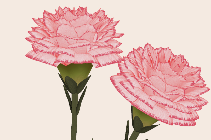
Generate a 3D visualization of carnation flowers
with sepals and stems for celebrating Mother's Day 2026.

function carnation
% CARNATION Generate a 3D visualization of carnation flowers with sepals and stems.
% This code is authored by Zhaoxu Liu / slandarer
% for the purpose of celebrating Mother's Day 2026.
% =========================================================================
% Zhaoxu Liu / slandarer (2026). carnation for Mother's Day
% (https://www.mathworks.com/matlabcentral/fileexchange/183838-carnation-for-mother-s-day),
% MATLAB Central File Exchange. Retrieved May 9, 2026.
% Create figure and axes / 创建图窗及坐标区域
fig = figure('Units','normalized', 'Position',[.3,.1,.4,.8],'Color',[244,234,225]./255);
axes('Parent',fig, 'NextPlot','add', 'DataAspectRatio',[1,1,1],...
'View',[-64, 5.5], 'Position',[0,-.15,1,1], 'Color',[244,234,225]./255, ...
'XColor','none', 'YColor','none', 'ZColor','none');
annotation("textbox", [.05, .8, .9, .2], "String", {"Happy"; "Mother's Day"}, ...
'FontName','Segoe Script', 'FontSize',52, 'FontWeight','bold', 'EdgeColor','none', ...
'HorizontalAlignment','center', 'VerticalAlignment','middle', 'Color',[97,40,20]./255);
xx = linspace(0, 1, 100);
tt = linspace(0, 1, 1e4);
[X, P] = meshgrid(xx, tt);
T1 = P*20*pi;
C1 = 1 - (1 - mod(3.6*T1/pi, 2)).^4./2; % Petal profile / 花瓣形状
S1 = (sin(50*T1)/150 + sin(10*T1)/30).*min(1, max(0, (X - .85)/.1)); % Edge serration / 边缘褶皱和锯齿
Y1 = (- (X.*1.2 - .5).^5.*32 - 1)./15.*P; % Petal curvature / 花瓣弧度
% Petal shape and serration modeling + rotating the planar petal to tilt it
% 花瓣形状和锯齿塑造 + 转动平躺的花瓣令其倾斜
R1 = (C1 + S1).*(X.*sin(P) - Y1.*cos(P))./(P + .5);
H1 = (C1 + S1).*(X.*cos(P) + Y1.*sin(P));
% Convert radius to Cartesian coordinates / 将半径映射为X,Y坐标
X1 = R1.*cos(T1);
Y1 = R1.*sin(T1);
% Colormap for carnation petals / 康乃馨配色
CList1 = [208, 62, 23; 221,146,121; 229,201,202; 233,219,222; 237,223,225]./255;
CMat1 = zeros(1e4, 100, 3);
CMat1(:, :, 1) = repmat(interp1(linspace(0, 1, size(CList1, 1)), CList1(:, 1), linspace(0, 1, 100)), [1e4, 1]);
CMat1(:, :, 2) = repmat(interp1(linspace(0, 1, size(CList1, 1)), CList1(:, 2), linspace(0, 1, 100)), [1e4, 1]);
CMat1(:, :, 3) = repmat(interp1(linspace(0, 1, size(CList1, 1)), CList1(:, 3), linspace(0, 1, 100)), [1e4, 1]);
% Darken edges / 边缘的深色
for i = 1:1e4
tNum = randi([98, 100]);
CMat1(i, tNum:end, 1) = 212./255;
CMat1(i, tNum:end, 2) = 87./255;
CMat1(i, tNum:end, 3) = 113./255;
end
% Rotation matrices / 旋转矩阵
Rx = @(rx) [1, 0, 0; 0, cos(rx), -sin(rx); 0, sin(rx), cos(rx)];
Rz = @(yz) [cos(yz), - sin(yz), 0; sin(yz), cos(yz), 0; 0, 0, 1];
Rx1 = Rx(pi/6); Rz1 = Rz(0);
% Render flower / 绘制康乃馨
surface(X1, Y1, H1 + .3, 'CData',CMat1, 'EdgeAlpha',0.1, 'EdgeColor',[224,39,39]./255, 'FaceColor','interp')
[U1, V1, W1] = matRotate(X1, Y1, H1 + .3, Rx1);
surface(U1 + .7, V1 - .7, W1 - .6, 'CData',CMat1, 'EdgeAlpha',0.1, 'EdgeColor',[224,39,39]./255, 'FaceColor','interp')
% Following the same method as before,
% the profile is designed with four serrated cycles to simulate the four sepals.
% 还是之前的方法,不过让轮廓有4个锯齿状周期来模拟四片花萼
% Sepals generation with 4-lobed pattern / 生成四片花萼(带4个锯齿状周期)
[X, T] = meshgrid(linspace(0, 1, 100), linspace(0, 1, 100).*2*pi);
P2 = T.*0 + pi/8;
C2 = .5 + (.5 - abs(mod(T, pi/2)/pi*2 - .5))*.4;
Y2 = (- (X.*1 - .5).^7.*128 - 1)./15 - .1;
R2 = C2.*(X.*sin(P2) - Y2.*cos(P2));
H2 = C2.*(X.*cos(P2) + Y2.*sin(P2));
X2 = R2.*cos(T);
Y2 = R2.*sin(T);
% Rotate by 90 degrees around the z-axis
% and reduce the size to render the four smaller sepals.
% 绕z轴旋转90度且减小其大小,绘制四片小花萼
% Smaller sepal layer / 绘制四片小花萼(第二层)
P3 = T.*0 + pi/10;
C3 = .3 + (.5 - abs(mod(T + pi/4, pi/2)/pi*2 - .5))*.7;
Y3 = (- (X.*.7 - .5).^7.*128 - 1)./15 - .1;
R3 = C3.*(X.*sin(P3) - Y3.*cos(P3));
H3 = C3.*(X.*cos(P3) + Y3.*sin(P3));
X3 = R3.*cos(T);
Y3 = R3.*sin(T);
% Colormap for sepals / 花托配色
CList2 = [178,173,113; 151,135, 73; 117,123, 50; 86, 89, 29; 75, 65, 17]./255;
CMat2 = zeros(100, 100, 3);
CMat2(:, :, 1) = repmat(interp1(linspace(0, 1, size(CList2, 1)), CList2(:, 1), linspace(0, 1, 100)), [100, 1]);
CMat2(:, :, 2) = repmat(interp1(linspace(0, 1, size(CList2, 1)), CList2(:, 2), linspace(0, 1, 100)), [100, 1]);
CMat2(:, :, 3) = repmat(interp1(linspace(0, 1, size(CList2, 1)), CList2(:, 3), linspace(0, 1, 100)), [100, 1]);
% Render sepals / 绘制花托
surf(X2, Y2, H2.*.8 + .12, 'CData',CMat2, 'EdgeAlpha',0.1, 'EdgeColor',CList2(end,:), 'FaceColor','interp')
surf(X3.*.93, Y3.*.92, H3.*.5 + .02, 'FaceColor',[ 84, 85, 54]./255, 'EdgeAlpha',0.1, 'EdgeColor','k')
[U2, V2, W2] = matRotate(X2, Y2, H2.*.8 + .12, Rx1);
[U3, V3, W3] = matRotate(X3.*.93, Y3.*.92, H3.*.5 + .02, Rx1);
surf(U2 + .7, V2 - .7, W2 - .6, 'CData',CMat2, 'EdgeAlpha',0.1, 'EdgeColor',CList2(end,:), 'FaceColor','interp')
surf(U3 + .7, V3 - .7, W3 - .6, 'FaceColor',[ 84, 85, 54]./255, 'EdgeAlpha',0.1, 'EdgeColor','k')
% A pulse function with two periods is applied
% to the contour to simulate the leaves.
% 让轮廓有2个周期且是脉冲函数,来模拟叶片
P4 = T.*0 + pi/16;
C4 = - abs(mod(T, pi)/pi - .5) + .11;
C4(C4 < 0) = 0; C4 = C4.*10; C4(51:100, :) = C4(51:100, :).*.7;
Y4 = (- (X.*1.01 - .5).^7.*128 - 1)./15 - .03;
R4 = C4.*(X.*sin(P4) - Y4.*cos(P4));
H4 = C4.*(X.*cos(P4) + Y4.*sin(P4));
X4 = R4.*cos(T);
Y4 = R4.*sin(T);
surf(X4 - .1, Y4 + .05, H4 - 2.2, 'FaceColor',[ 84, 85, 54]./255, 'EdgeAlpha',0.1, 'EdgeColor','k')
[U4, V4, W4] = matRotate(X4 - .1, Y4 - .1, H4 + .1, Rz1);
[U4, V4, W4] = matRotate(U4, V4, W4, Rx1);
surf(U4 + .7, V4 - .7 + 1, W4 - .6 - 1.2, 'FaceColor',[ 84, 85, 54]./255, 'EdgeAlpha',0.1, 'EdgeColor','k')
P5 = T.*0 + pi/8;
C5 = - abs(mod(T + pi/6, pi)/pi - .5) + .11;
C5(C5 < 0) = 0; C5 = C5.*5;
Y5 = (- (X.*1.01 - .5).^7.*128 - 1)./15 - .1;
R5 = C5.*(X.*sin(P5) - Y5.*cos(P5));
H5 = C5.*(X.*cos(P5) + Y5.*sin(P5));
X5 = R5.*cos(T);
Y5 = R5.*sin(T);
surf(X5, Y5, H5 - .3, 'FaceColor',[ 84, 85, 54]./255, 'EdgeAlpha',0.1, 'EdgeColor','k')
[U5, V5, W5] = matRotate(X5, Y5, H5+.1, Rx1);
surf(U5 + .7, V5 - .7 + 1/4, W5 - .6 - 1.7/4, 'FaceColor',[ 84, 85, 54]./255, 'EdgeAlpha',0.1, 'EdgeColor','k')
% Render stems / 绘制花杆
P1_1 = [mean(X3(:).*.93), mean(Y3(:).*.92), mean(H3(:).*.5 + .02)];
P1_2 = [mean(X5(:)), mean(Y5(:)), mean(H5(:) - .3)];
P1_3 = [mean(X4(:) - .1), mean(Y4(:) + .05), mean(H4(:) - 2.2)];
P1_3 = (P1_3 - P1_2).*1.4 + P1_2;
[XX1, YY1, ZZ1] = cylinderXYZ(P1_1, P1_2, .05);
[XX2, YY2, ZZ2] = cylinderXYZ(P1_2, P1_3, .04);
surf(XX1, YY1, ZZ1, 'FaceColor',[ 84, 85, 54]./255, 'EdgeAlpha',0.1, 'EdgeColor','k')
surf(XX2, YY2, ZZ2, 'FaceColor',[ 84, 85, 54]./255, 'EdgeAlpha',0.1, 'EdgeColor','k')
P1_1 = [mean(U3(:) + .7), mean(V3(:) - .7), mean(W3(:) - .6)];
P1_2 = [mean(U5(:) + .7), mean(V5(:) - .7 + 1/4), mean(W5(:) - .6 - 1.7/4)];
P1_3 = [mean(U4(:) + .7), mean(V4(:) - .7 + 1), mean(W4(:) - .6 - 1.2)];
P1_3 = (P1_3 - P1_2).*2.4 + P1_2;
[XX1, YY1, ZZ1] = cylinderXYZ(P1_1, P1_2, .05);
[XX2, YY2, ZZ2] = cylinderXYZ(P1_2, P1_3, .04);
surf(XX1, YY1, ZZ1, 'FaceColor',[ 84, 85, 54]./255, 'EdgeAlpha',0.1, 'EdgeColor','k')
surf(XX2, YY2, ZZ2, 'FaceColor',[ 84, 85, 54]./255, 'EdgeAlpha',0.1, 'EdgeColor','k')
% 在任意两点间构建圆柱
function [XX, YY, ZZ] = cylinderXYZ(P1, P2, r)
% CYLINDERXYZ Create a cylinder connecting two 3D points
% [XX, YY, ZZ] = cylinderXYZ(P1, P2, r) generates a cylinder
% of radius r between points P1 and P2.
v = P2 - P1; l = norm(v);
if l < eps, return; end
[XX, YY, ZZ] = cylinder(r, 30); ZZ = ZZ * l;
ddir = [0, 0, 1]; tdir = v / l;
if dot(ddir, tdir) > 0.9999
R = eye(3);
elseif dot(ddir, tdir) < -0.9999
R = [1, 0, 0; 0, -1, 0; 0, 0, -1];
else
av = cross(ddir, tdir); av = av / norm(av);
R = axisRotate(av, acos(dot(ddir, tdir)));
end
for ii = 1:size(XX, 1)
for jj = 1:size(XX, 2)
p = R * [XX(ii, jj); YY(ii, jj); ZZ(ii, jj)];
XX(ii, jj) = p(1) + P1(1);
YY(ii, jj) = p(2) + P1(2);
ZZ(ii, jj) = p(3) + P1(3);
end
end
end
% 通过矩阵旋转数据
function [U, V, W] = matRotate(X, Y, Z, R)
% MATROTATE Apply 3x3 rotation matrix to a set of 3D points
% [U,V,W] = matRotate(X,Y,Z,R) rotates points (X,Y,Z)
% using rotation matrix R.
U = X; V = Y; W = Z;
for ii = 1:numel(X)
v = [X(ii); Y(ii); Z(ii)];
n = R*v; U(ii) = n(1); V(ii) = n(2); W(ii) = n(3);
end
end
% 根据轴-角参数生成旋转矩阵
function R = axisRotate(axis, angle)
% AXISROTATE Compute rotation matrix from axis-angle representation
% R = axisRotate(axis, angle) returns a 3x3 rotation matrix
% for rotating by angle (radians) around the given axis vector.
% Implementation based on Rodrigues' rotation formula.
u = axis(1); v = axis(2); w = axis(3);
c = cos(angle); s = sin(angle);
R = [u^2 + (1-u^2)*c, u*v*(1-c) - w*s, u*w*(1-c) + v*s;
u*v*(1-c) + w*s, v^2 + (1-v^2)*c, v*w*(1-c) - u*s;
u*w*(1-c) - v*s, v*w*(1-c) + u*s, w^2 + (1-w^2)*c];
end
end
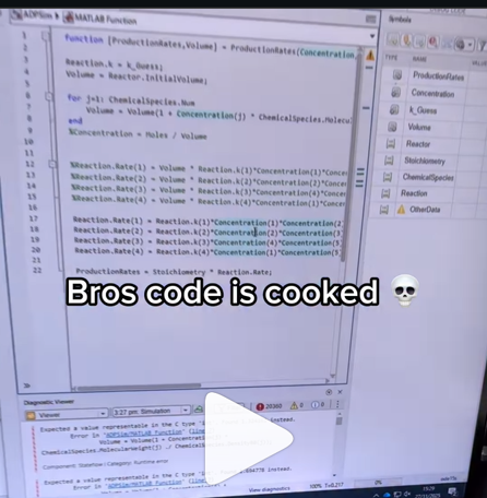
A coworker shared with me a hilarious Instagram post today. A brave bro posted a short video showing his MATLAB code… casually throwing 49,000 errors!
Surprisingly, the video went virial and recieved 250,000+ likes and 800+ comments. You really never know what the Instagram algorithm is thinking, but apparently “my code is absolutely cooked” is a universal developer experience 😂
Last note: Can someone please help this Bro fix his code?

The formula comes from @yuruyurau. (https://x.com/yuruyurau)
digital life 1

figure('Position',[300,50,900,900], 'Color','k');
axes(gcf, 'NextPlot','add', 'Position',[0,0,1,1], 'Color','k');
axis([0, 400, 0, 400])
SHdl = scatter([], [], 2, 'filled','o','w', 'MarkerEdgeColor','none', 'MarkerFaceAlpha',.4);
t = 0;
i = 0:2e4;
x = mod(i, 100);
y = floor(i./100);
k = x./4 - 12.5;
e = y./9 + 5;
o = vecnorm([k; e])./9;
while true
t = t + pi/90;
q = x + 99 + tan(1./k) + o.*k.*(cos(e.*9)./4 + cos(y./2)).*sin(o.*4 - t);
c = o.*e./30 - t./8;
SHdl.XData = (q.*0.7.*sin(c)) + 9.*cos(y./19 + t) + 200;
SHdl.YData = 200 + (q./2.*cos(c));
drawnow
end
digital life 2

figure('Position',[300,50,900,900], 'Color','k');
axes(gcf, 'NextPlot','add', 'Position',[0,0,1,1], 'Color','k');
axis([0, 400, 0, 400])
SHdl = scatter([], [], 2, 'filled','o','w', 'MarkerEdgeColor','none', 'MarkerFaceAlpha',.4);
t = 0;
i = 0:1e4;
x = i;
y = i./235;
e = y./8 - 13;
while true
t = t + pi/240;
k = (4 + sin(y.*2 - t).*3).*cos(x./29);
d = vecnorm([k; e]);
q = 3.*sin(k.*2) + 0.3./k + sin(y./25).*k.*(9 + 4.*sin(e.*9 - d.*3 + t.*2));
SHdl.XData = q + 30.*cos(d - t) + 200;
SHdl.YData = 620 - q.*sin(d - t) - d.*39;
drawnow
end
digital life 3

figure('Position',[300,50,900,900], 'Color','k');
axes(gcf, 'NextPlot','add', 'Position',[0,0,1,1], 'Color','k');
axis([0, 400, 0, 400])
SHdl = scatter([], [], 1, 'filled','o','w', 'MarkerEdgeColor','none', 'MarkerFaceAlpha',.4);
t = 0;
i = 0:1e4;
x = mod(i, 200);
y = i./43;
k = 5.*cos(x./14).*cos(y./30);
e = y./8 - 13;
d = (k.^2 + e.^2)./59 + 4;
a = atan2(k, e);
while true
t = t + pi/20;
q = 60 - 3.*sin(a.*e) + k.*(3 + 4./d.*sin(d.^2 - t.*2));
c = d./2 + e./99 - t./18;
SHdl.XData = q.*sin(c) + 200;
SHdl.YData = (q + d.*9).*cos(c) + 200;
drawnow; pause(1e-2)
end
digital life 4

figure('Position',[300,50,900,900], 'Color','k');
axes(gcf, 'NextPlot','add', 'Position',[0,0,1,1], 'Color','k');
axis([0, 400, 0, 400])
SHdl = scatter([], [], 1, 'filled','o','w', 'MarkerEdgeColor','none', 'MarkerFaceAlpha',.4);
t = 0;
i = 0:4e4;
x = mod(i, 200);
y = i./200;
k = x./8 - 12.5;
e = y./8 - 12.5;
o = (k.^2 + e.^2)./169;
d = .5 + 5.*cos(o);
while true
t = t + pi/120;
SHdl.XData = x + d.*k.*sin(d.*2 + o + t) + e.*cos(e + t) + 100;
SHdl.YData = y./4 - o.*135 + d.*6.*cos(d.*3 + o.*9 + t) + 275;
SHdl.CData = ((d.*sin(k).*sin(t.*4 + e)).^2).'.*[1,1,1];
drawnow;
end
digital life 5

figure('Position',[300,50,900,900], 'Color','k');
axes(gcf, 'NextPlot','add', 'Position',[0,0,1,1], 'Color','k');
axis([0, 400, 0, 400])
SHdl = scatter([], [], 1, 'filled','o','w',...
'MarkerEdgeColor','none', 'MarkerFaceAlpha',.4);
t = 0;
i = 0:1e4;
x = mod(i, 200);
y = i./55;
k = 9.*cos(x./8);
e = y./8 - 12.5;
while true
t = t + pi/120;
d = (k.^2 + e.^2)./99 + sin(t)./6 + .5;
q = 99 - e.*sin(atan2(k, e).*7)./d + k.*(3 + cos(d.^2 - t).*2);
c = d./2 + e./69 - t./16;
SHdl.XData = q.*sin(c) + 200;
SHdl.YData = (q + 19.*d).*cos(c) + 200;
drawnow;
end
digital life 6

clc; clear
figure('Position',[300,50,900,900], 'Color','k');
axes(gcf, 'NextPlot','add', 'Position',[0,0,1,1], 'Color','k');
axis([0, 400, 0, 400])
SHdl = scatter([], [], 2, 'filled','o','w', 'MarkerEdgeColor','none', 'MarkerFaceAlpha',.4);
t = 0;
i = 1:1e4;
y = i./790;
k = y; idx = y < 5;
k(idx) = 6 + sin(bitxor(floor(y(idx)), 1)).*6;
k(~idx) = 4 + cos(y(~idx));
while true
t = t + pi/90;
d = sqrt((k.*cos(i + t./4)).^2 + (y/3-13).^2);
q = y.*k.*cos(i + t./4)./5.*(2 + sin(d.*2 + y - t.*4));
c = d./3 - t./2 + mod(i, 2);
SHdl.XData = q + 90.*cos(c) + 200;
SHdl.YData = 400 - (q.*sin(c) + d.*29 - 170);
drawnow; pause(1e-2)
end
digital life 7

clc; clear
figure('Position',[300,50,900,900], 'Color','k');
axes(gcf, 'NextPlot','add', 'Position',[0,0,1,1], 'Color','k');
axis([0, 400, 0, 400])
SHdl = scatter([], [], 2, 'filled','o','w', 'MarkerEdgeColor','none', 'MarkerFaceAlpha',.4);
t = 0;
i = 1:1e4;
y = i./345;
x = y; idx = y < 11;
x(idx) = 6 + sin(bitxor(floor(x(idx)), 8))*6;
x(~idx) = x(~idx)./5 + cos(x(~idx)./2);
e = y./7 - 13;
while true
t = t + pi/120;
k = x.*cos(i - t./4);
d = sqrt(k.^2 + e.^2) + sin(e./4 + t)./2;
q = y.*k./d.*(3 + sin(d.*2 + y./2 - t.*4));
c = d./2 + 1 - t./2;
SHdl.XData = q + 60.*cos(c) + 200;
SHdl.YData = 400 - (q.*sin(c) + d.*29 - 170);
drawnow; pause(5e-3)
end
digital life 8

clc; clear
figure('Position',[300,50,900,900], 'Color','k');
axes(gcf, 'NextPlot','add', 'Position',[0,0,1,1], 'Color','k');
axis([0, 400, 0, 400])
SHdl{6} = [];
for j = 1:6
SHdl{j} = scatter([], [], 2, 'filled','o','w', 'MarkerEdgeColor','none', 'MarkerFaceAlpha',.3);
end
t = 0;
i = 1:2e4;
k = mod(i, 25) - 12;
e = i./800; m = 200;
theta = pi/3;
R = [cos(theta) -sin(theta); sin(theta) cos(theta)];
while true
t = t + pi/240;
d = 7.*cos(sqrt(k.^2 + e.^2)./3 + t./2);
XY = [k.*4 + d.*k.*sin(d + e./9 + t);
e.*2 - d.*9 - d.*9.*cos(d + t)];
for j = 1:6
XY = R*XY;
SHdl{j}.XData = XY(1,:) + m;
SHdl{j}.YData = XY(2,:) + m;
end
drawnow;
end
digital life 9

clc; clear
figure('Position',[300,50,900,900], 'Color','k');
axes(gcf, 'NextPlot','add', 'Position',[0,0,1,1], 'Color','k');
axis([0, 400, 0, 400])
SHdl{14} = [];
for j = 1:14
SHdl{j} = scatter([], [], 2, 'filled','o','w', 'MarkerEdgeColor','none', 'MarkerFaceAlpha',.1);
end
t = 0;
i = 1:2e4;
k = mod(i, 50) - 25;
e = i./1100; m = 200;
theta = pi/7;
R = [cos(theta) -sin(theta); sin(theta) cos(theta)];
while true
t = t + pi/240;
d = 5.*cos(sqrt(k.^2 + e.^2) - t + mod(i, 2));
XY = [k + k.*d./6.*sin(d + e./3 + t);
90 + e.*d - e./d.*2.*cos(d + t)];
for j = 1:14
XY = R*XY;
SHdl{j}.XData = XY(1,:) + m;
SHdl{j}.YData = XY(2,:) + m;
end
drawnow;
end
Pure Matlab
82%
Simulink
18%
11 votes
Jorge Bernal-AlvizJorge Bernal-Alviz shared the following code that requires R2025a or later:
Test()

function Test()
duration = 10;
numFrames = 800;
frameInterval = duration / numFrames;
w = 400;
t = 0;
i_vals = 1:10000;
x_vals = i_vals;
y_vals = i_vals / 235;
r = linspace(0, 1, 300)';
g = linspace(0, 0.1, 300)';
b = linspace(1, 0, 300)';
r = r * 0.8 + 0.1;
g = g * 0.6 + 0.1;
b = b * 0.9 + 0.1;
customColormap = [r, g, b];
figure('Position', [100, 100, w, w], 'Color', [0, 0, 0]);
axis equal;
axis off;
xlim([0, w]);
ylim([0, w]);
hold on;
colormap default;
colormap(customColormap);
plothandle = scatter([], [], 1, 'filled', 'MarkerFaceAlpha', 0.12);
for i = 1:numFrames
t = t + pi/240;
k = (4 + 3 * sin(y_vals * 2 - t)) .* cos(x_vals / 29);
e = y_vals / 8 - 13;
d = sqrt(k.^2 + e.^2);
c = d - t;
q = 3 * sin(2 * k) + 0.3 ./ (k + 1e-10) + ...
sin(y_vals / 25) .* k .* (9 + 4 * sin(9 * e - 3 * d + 2 * t));
points_x = q + 30 * cos(c) + 200;
points_y = q .* sin(c) + 39 * d - 220;
points_y = w - points_y;
CData = (1 + sin(0.1 * (d - t))) / 3;
CData = max(0, min(1, CData));
set(plothandle, 'XData', points_x, 'YData', points_y, 'CData', CData);
brightness = 0.5 + 0.3 * sin(t * 0.2);
set(plothandle, 'MarkerFaceAlpha', brightness);
drawnow;
pause(frameInterval);
end
end
I came across this fun video from @Christoper Lum, and I have to admit—his MathWorks swag collection is pretty impressive! He’s got pieces I even don’t have.
So now I’m curious… what MathWorks swag do you have hiding in your office or closet?
- Which one is your favorite?
- Which ones do you want to add to your collection?
Show off your swag and share it with the community! 🚀
Inspired by @xingxingcui's post about old MATLAB versions and @유장's post about an old Easter egg, I thought it might be fun to share some MATLAB-Old-Timer Stories™.
Back in the early 90s, MATLAB had been ported to MacOS, but there were some interesting wrinkles. One that kept me earning my money as a computer lab tutor was that MATLAB required file names to follow Windows standards - no spaces or other special characters. But on a Mac, nothing stopped you from naming your script "hello world - 123.m". The problem came when you tried to run it. MATLAB was essentially doing an eval on the script name, assuming the file name would follow Windows (and MATLAB) naming rules.
So now imagine a lab full of students taking a university course. As is common in many universities, the course was given a numeric code. For whatever historical reason, my school at that time was also using numeric codes for the departments. Despite being told the rules for naming scripts, many students would default to something like "26.165 - 1.1" for problem one on HW1 for the intro applied math course 26.165.
No matter what they did in their script, when they ran it, MATLAB would just say "ans = 25.0650".
Nothing brings you more MATLAB-god credibility as a student tutor than walking over to someone's computer, taking one look at their output, saying "rename your file", and walking away like a boss.
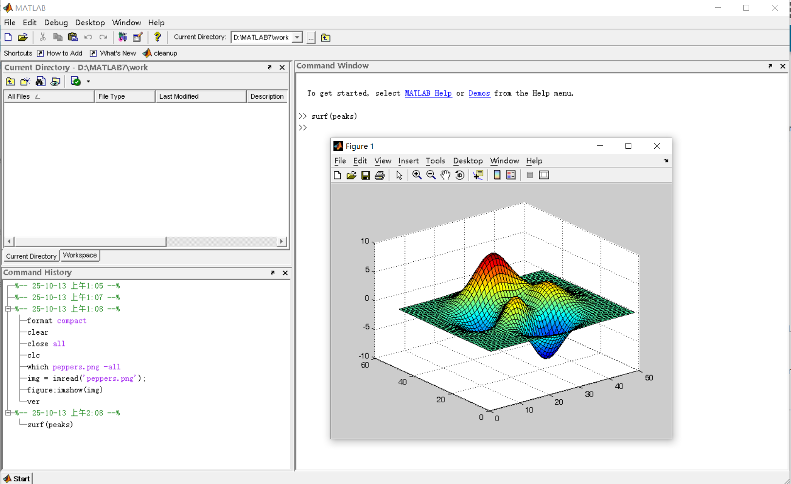
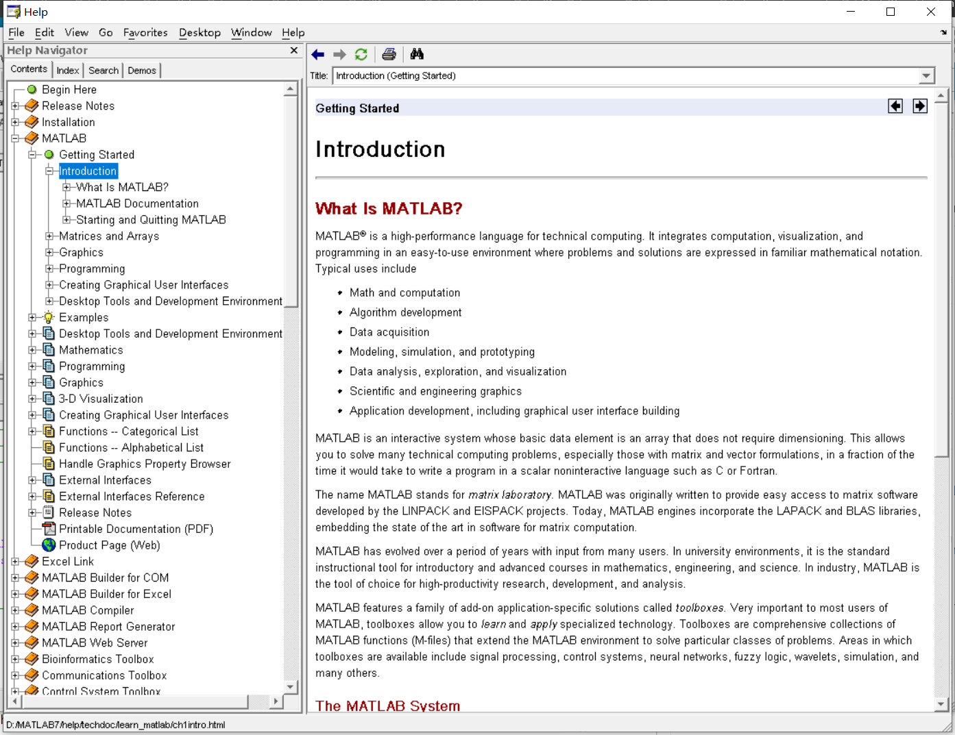
It was 2010 when I was a sophomore in university. I chose to learn MATLAB because of a mathematical modeling competition, and the university provided MATLAB 7.0, a very classic release. To get started, I borrowed many MATLAB books from the library and began by learning simple numerical calculations, plotting, and solving equations. Gradually I was drawn in by MATLAB’s powerful capabilities and became interested; I often used it as a big calculator for fun. That version didn’t have MATLAB Live Script; instead it used MATLAB Notebook (M-Book), which allowed MATLAB functions to be used directly within Microsoft Word, and it also had the Symbolic Math Toolbox’s MuPAD interactive environment. These were later gradually replaced by Live Scripts introduced in R2016a. There are many similar examples...
Out of curiosity, I still have screenshots on my computer showing MATLAB 7.0 running compatibly. I’d love to hear your thoughts?

Do you have a swag signed by Brian Douglas? He does!
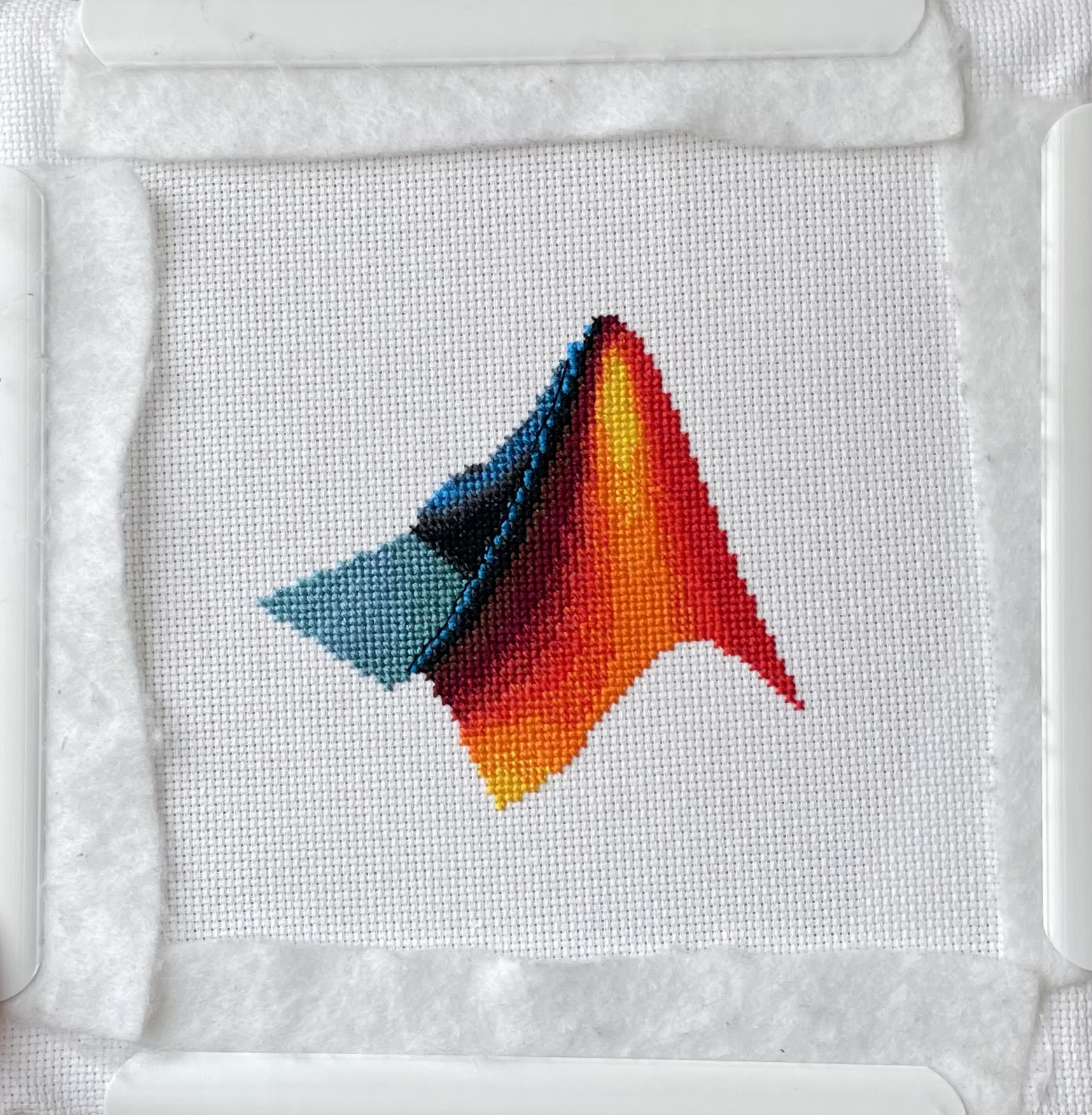
I designed and stitched this last week! It uses a total of 20 DMC thread colors, and I frequently stitched with two colors at once to create the gradient.
I saw this on Reddit and thought of the past mini-hack contests. We have a few folks here who can do something similar with MATLAB.
I saw this YouTube short on my feed: What is MATLab?

I was mostly mesmerized by the minecraft gameplay going on in the background.
Found it funny, thought i'd share.
Trinity
- It's the question that drives us, Neo. It's the question that brought you here. You know the question, just as I did.
Neo
- What is the Matlab?
Morpheus
- Unfortunately, no one can be told what the Matlab is. You have to see it for yourself.
And also later :
Morpheus
- The Matlab is everywhere. It is all around us. Even now, in this very room. You can feel it when you go to work [...]
The Architect
- The first Matlab I designed was quite naturally perfect. It was a work of art. Flawless. Sublime.
[My Matlab quotes version of the movie (Matrix, 1999) ]
Resharing a fun short video explaining what MATLAB is. :)
Hey MATLAB enthusiasts!
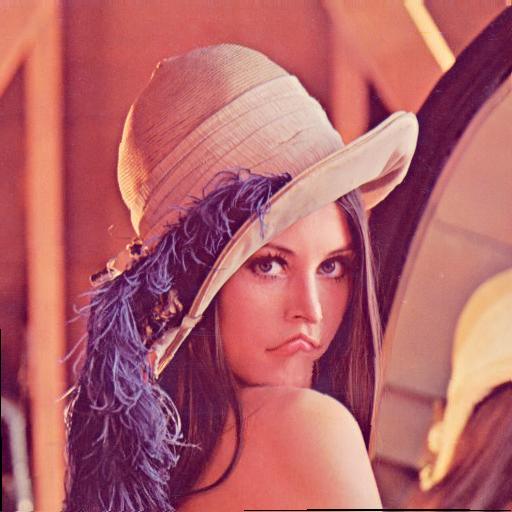
I just stumbled upon this hilariously effective GitHub repo for image deformation using Moving Least Squares (MLS)—and it’s pure gold for anyone who loves playing with pixels! 🎨✨
- Real-Time Magic ✨
- Precomputes weights and deformation data upfront, making it blazing fast for interactive edits. Drag control points and watch the image warp like rubber! (2)
- Supports affine, similarity, and rigid deformations—because why settle for one flavor of chaos?
- Single-File Simplicity 🧩
- All packed into one clean MATLAB class (mlsImageWarp.m).
- Endless Fun Use Cases 🤹
- Turn your pet’s photo into a Picasso painting.
- "Fix" your friend’s smile... aggressively.
- Animate static images with silly deformations (1).
Try the Demo!
You are not a jedi yet !
20%
We not grant u the rank of master !
0%
Ready are u? What knows u of ready?
0%
May the Force be with you !
80%
5 votes
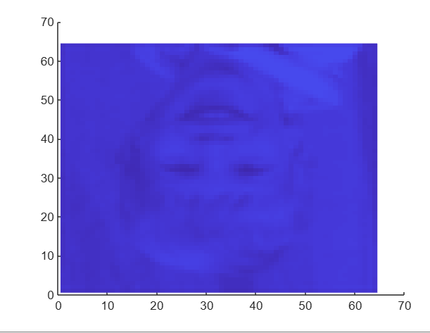
I had an error in the web version Matlab, so I exited and came back in, and this boy was plotted.
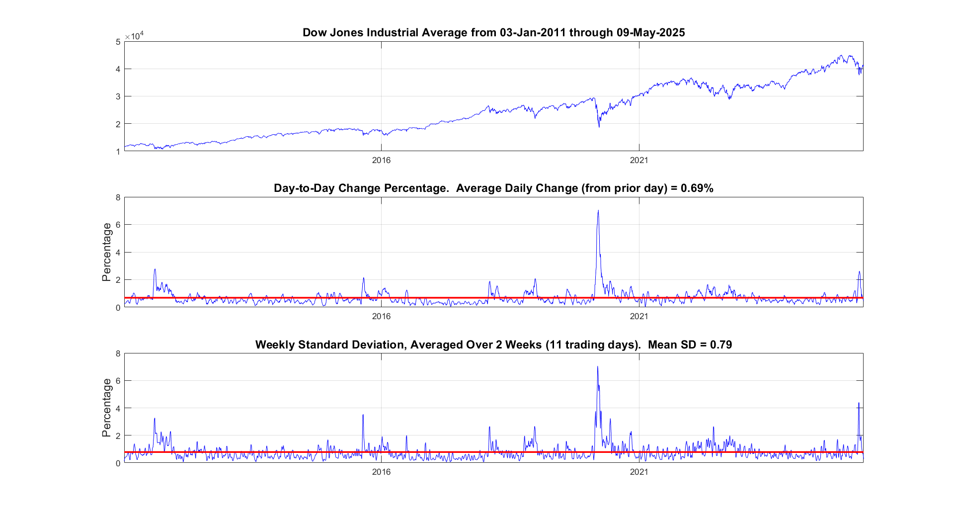
It seems like the financial news is always saying the stock market is especially volatile now. But is it really? This code will show you the daily variation from the prior day. You can see that the average daily change from one day to the next is 0.69%. So any change in the stock market from the prior day less than about 0.7% or 1% is just normal "noise"/typical variation. You can modify the code to adjust the starting date for the analysis. Data file (Excel workbook) is attached (hopefully - I attached it twice but it's not showing up yet).
% Program to plot the Dow Jones Industrial Average from 1928 to May 2025, and compute the standard deviation.
% Data available for download at https://finance.yahoo.com/quote/%5EDJI/history?p=%5EDJI
% Just set the Time Period, then find and click the download link, but you ned a paid version of Yahoo.
%
% If you have a subscription for Microsoft Office 365, you can also get historical stock prices.
% Reference: https://support.microsoft.com/en-us/office/stockhistory-function-1ac8b5b3-5f62-4d94-8ab8-7504ec7239a8#:~:text=The%20STOCKHISTORY%20function%20retrieves%20historical,Microsoft%20365%20Business%20Premium%20subscription.
% For example put this in an Excel Cell
% =STOCKHISTORY("^DJI", "1/1/2000", "5/10/2025", 0, 1, 0, 1,2,3,4, 5)
% and it will fill out a table in Excel
%====================================================================================================================
clc; % Clear the command window.
close all; % Close all figures (except those of imtool.)
imtool close all; % Close all imtool figures if you have the Image Processing Toolbox.
clear; % Erase all existing variables. Or clearvars if you want.
workspace; % Make sure the workspace panel is showing.
format long g;
format compact;
fontSize = 14;
filename = 'Dow Jones Industrial Index.xlsx';
data = readtable(filename);
% Date,Close,Open,High,Low,Volume
dates = data.Date;
closing = data.Close;
volume = data.Volume;
% Define start date and stop date
startDate = datetime(2011,1,1)
stopDate = dates(end)
selectedDates = dates > startDate;
% Extract those dates:
dates = dates(selectedDates);
closing = closing(selectedDates);
volume = volume(selectedDates);
% Plot Volume
hFigVolume = figure('Name', 'Daily Volume');
plot(dates, volume, 'b-');
grid on;
xticks(startDate:calendarDuration(5,0,0):stopDate)
title('Dow Jones Industrial Average Volume', 'FontSize', fontSize);
hFig = figure('Name', 'Daily Standard Deviation');
subplot(3, 1, 1);
plot(dates, closing, 'b-');
xticks(startDate:calendarDuration(5,0,0):stopDate)
drawnow;
grid on;
caption = sprintf('Dow Jones Industrial Average from %s through %s', dates(1), dates(end));
title(caption, 'FontSize', fontSize);
% Get the average change from one trading day to the next.
diffs = 100 * abs(closing(2:end) - closing(1:end-1)) ./ closing(1:end-1);
subplot(3, 1, 2);
averageDailyChange = mean(diffs)
% Looks pretty noisy so let's smooth it for a nicer display.
numWeeks = 4;
diffs = sgolayfilt(diffs, 2, 5*numWeeks+1);
plot(dates(2:end), diffs, 'b-');
grid on;
xticks(startDate:calendarDuration(5,0,0):stopDate)
hold on;
line(xlim, [averageDailyChange, averageDailyChange], 'Color', 'r', 'LineWidth', 2);
ylabel('Percentage', 'FontSize', fontSize);
caption = sprintf('Day-to-Day Change Percentage. Average Daily Change (from prior day) = %.2f%%', averageDailyChange);
title(caption, 'FontSize', fontSize);
drawnow;
% Get the stddev over a 5 trading day window.
sd = stdfilt(closing, ones(5, 1));
% Get it relative to the magnitude.
sd = sd ./ closing * 100;
averageVariation = mean(sd)
numWeeks = 2;
% Looks pretty noisy so let's smooth it for a nicer display.
sd = sgolayfilt(sd, 2, 5*numWeeks+1);
% Plot it.
subplot(3, 1, 3);
plot(dates, sd, 'b-');
grid on;
xticks(startDate:calendarDuration(5,0,0):stopDate)
hold on;
line(xlim, [averageVariation, averageVariation], 'Color', 'r', 'LineWidth', 2);
ylabel('Percentage', 'FontSize', fontSize);
caption = sprintf('Weekly Standard Deviation, Averaged Over %d Weeks (%d trading days). Mean SD = %.2f', ...
numWeeks, 5*numWeeks+1, averageVariation);
title(caption, 'FontSize', fontSize);
% Maximize figure window.
g = gcf;
g.WindowState = 'maximized';