Results for
Short version: MathWorks have released the MATLAB Agentic Toolkit which will significantly improve the life of anyone who is using MATLAB and Simulink with agentic AI systems such as Claude Code or OpenAI Codex. Go and get it from here: https://github.com/matlab/matlab-agentic-toolkit
Long version: On The MATLAB Blog Introducing the MATLAB Agentic Toolkit » The MATLAB Blog - MATLAB & Simulink
MATLAB EXPO India | 7 May | Bengaluru
Get inspired by the latest trends and real-world customer success stories transforming industries. Learn from trusted experts across 4 tracks.
- AI & Autonomous Systems
- Electrification
- Systems & Software Engineering
- Radar, Wireless & HDL
Register at bit.ly/matlabexpocommunity

Do we know if MATLAB is being used on the Artemis II (moon mission) spacecraft itself? Like is the crew running MATLAB programs? I imagine it was probably at least used in development of some of the components of the spacecraft, rockets, or launch building. Or is it used for any of the image analysis of the images collected by the spacecraft?
MATLAB interprets the first block of uninterupted comments in a function file as documentation. Consider a simple example.
% myfunc This is my function
%
% See also sin
function z = myfunc(x, y)
z = x + y;
end
Those comments are printed in the command window with "help myfunc" and displayed in a separate window with "doc myfunc". A lot of useful things happen behind the scenes as well.
- Hyperlinks are automatically added for valid file names after "See also".
- When dealing with classes, the doc command automatically appends the comment block with a lists of properties and methods.
All this is very handy and as been around for quite some time. However, the doc browser isn't great (forward/back feature was removed several versons ago), the text formatting isn't great, and there is no way to display math.
Although pretty text/math can be displayed in a live document, the traditional *.mlx file format does not always play nice with Git and I have avoided them. However, live documents can now (since 2025a?) be saved in a pure text format, so I began to wonder if all functions should be written in this style. Turns out that all you have to do is append these lines:
%[appendix]{"version":"1.0"}
%---
to the end of any function file to make it a live function. Doing so changes how MATLAB manages that first comment block. The help command seems to be unaffacted, although [text] may appear at the start of each comment line (depending on if the file was create as a live function or subsequently converted). The doc command behaves very different: instead of bringing up the traditional window for custom documentation, the comment block looks like it gets published to HTML and looks more similar to standard MATLAB help. This is a win in some ways, but the "See also" capabilitity is lost.
Curiously, the same text can be appended to the end of a class definition file with some affect. It does not change how the file shows up in the editor, but as in live functions, comments are published when using the doc command. So we are partway to something like a "live class", but not quite.
Should one stick with traditional *.m files or make everything live? Neither does a great job for functions/classes in a namespace--references must explicitly know absolute location in traditional functions, and there is no "See also" concept in a live function. Do we need a command, like cdoc (custom documentation), that pulls out the comment block, publishing formatted text to HTML while simultaneously resolving "See also" references as hyperlinks? If so, it would be great if there were other special commands like "See examples" that would automatically copy and then open an example script for the end user.
Hi all,
I'm a UX researcher here at MathWorks working on the MathWorks Central Community. We're testing a new feature to make it easier to ask a question, and we'd love to hear from community members like you.
Sessions will be next week. They are remote, up to 2 hours (often shorter), and participants receive a $100 stipend. If you're interested, you can click here to schedule.
Thanks in advance! Your feedback directly shapes what gets built.
--David, MathWorks UX Research
Digital Twin Development of PEARL Autonomous Surface System Thermal Management
The top session of the countdown showcases how the PEARL engineering team used a digital twin to solve real‑world thermal challenges in a solar‑powered autonomous marine platform operating in extreme environments. After thermal shutdown events in the field, the team built a model that predicts temperatures at multiple locations with ~1% accuracy, while balancing accuracy with model complexity.
Beyond the technology, this keynote delivers practical lessons for predictive modeling and digital twins that apply well beyond marine systems.
We hope you’ve enjoyed the Top 10 countdown series—and a big thank‑you to Olivier de Weck at Massachusetts Institute of Technology, for delivering such a compelling and insightful keynote.
🎥 If you missed it live, be sure to watch the recording to see why it earned the #1 spot at MATLAB EXPO 2026.

MATLAB EXPO India is Back!
This in-person events brings together engineers, scientists, and researchers to explore the latest trends in engineering and science, and discover new MATLAB and Simulink capabilities to apply to your work.
May 7, 2026 l Bengaluru
Register at bit.ly/matlabexpocommunity

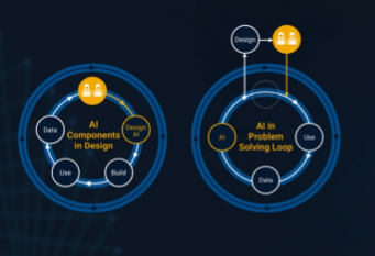
It’s no surprise this keynote landed at #2. MaryAnn Freeman, Senior Director of Engineering, AI, and Data Science explores how AI, especially generative AI, is transforming the way engineers design, build, and innovate. From accelerating the design loop with faster, data‑driven solutions, to blending human creativity with AI insights, to evolving engineering tools that turn ideas into build‑ready systems. This keynote shows how embedded intelligence helps engineers push past traditional limits and bridge imagination with real‑world impact.
If you’re curious about how AI is reshaping engineering workflows today (and what that means for the future of design), this is a must‑watch.
👉 Watch the keynote recording and see why it was one of the most popular sessions of MATLAB EXPO Online 2025.
Absolutely!
65%
Probably
9%
Sometimes yes, sometimes no
4%
Unlikely
17%
Never!
4%
23 votes
Matlab seems to follow a rule that iterative reduction operators give appropriate non-empty values to empty inputs. Examples include,
sum([])
prod([])
all([])
any([])
Is it an oversight not to do something similar for min and max?
max([])
For non-empty A and B,
max([A,B])= max(max(A), max(B))
The extension to B=[] should therefore satisfy,
max(A)=max(max(A),max([]))
for any A, which will only be true if we define max([])=-inf.
The 550,000th question has been asked on Answers.
Software‑defined vehicles are becoming reality—and this #3 ranked session shows how. In this keynote, Daniel Scurtu (NXP) demonstrates how MathWorks and NXP are working together to accelerate system‑level embedded development.
🔋 Using a vehicle electrification demo that runs across multiple NXP processors, you’ll see:
- Model‑Based Design workflows from concept to deployment
- Intelligent battery management and motor control
- Automatic code generation and hardware deployment
- ☁️ Real‑time cloud analytics and over‑the‑air updates
🛠️ Featuring MATLAB and Simulink products alongside NXP tools like Model-based Design Toolbox (MBDT), S32 Design Studio IDE, and Real-Time Drivers (RTD), this session highlights an end‑to‑end approach that reduces complexity and speeds the transition to software‑defined vehicles.
If you have published add-ons on File Exchange, you may have noticed that we recently added a new, unique package name field to all add-ons. This enables future support for automated installation with the MATLAB Package Manager. This name will be a unique identifier for your add-on and does not affect the existing add-on title, any file names, or the URL of your add-on.
📝 Update and review until April 10
We generated default package names for all add-ons. You can review and update the package name for your add-ons until April 10, 2026. Review your package names now:
After April 10, you will need to create a new version to change your package name.
🚀 More changes coming with the MATLAB R2026b prerelease
Starting with the MATLAB R2026b prerelease, these package names will take effect. At that time, the package name may appear on the File Exchange page for your add-on.
Keep your eyes peeled for exciting changes coming soon to your add-ons on File Exchange!
Cantera is an open-source suite of tools for problems involving chemical kinetics, thermodynamics, and transport processes. Dr. Su Sun, a recent graduate from Northeastern Chemical Engineering Ph.D. program made significant contributions to MATLAB interface for Cantera in Cantera Release 3.2.0 in collaboration with Dr. Richard West, other Cantera developers, and MathWorks Advanced Support and Development Teams. As part of this Release, MATLAB interface for Cantera transitioned to using the new MATLAB- C++ interface and expanded their unit testing. Further information is available here.
I began coding in MATLAB less than 2 months ago for a class at community college. Alongside the course content, I also completed the MATLAB onramp and introduction to linear algebra self-paced online courses. I think this is the most fun I've had coding since back when I used to make Scratch projects in elementary school. I'm kind of curious if I could recreate some of my favorite childhood Scratch games here.
Anyways, I just wanted to introduce myself since I plan to be really active this year. My name is Mehreen (meh like the meh emoji from the Emoji movie, reen like screen), I'm a data science undergrad sophomore from the U.S. and it's nice to meet you!
Hi everyone,
Some of you may remember my earlier post. Quick version: I'm a biomed PhD student, I use MATLAB daily, and I noticed that AI coding tools often suggest functions that don't exist in R2025b or use deprecated ones. So I built skills that teach them what actually works.
v2.0 adds 54 template `.m` scripts, rewrites all knowledge cards based on blind testing, and verifies every function call against live MATLAB. I tested each skill on 17 prompts and caught 8 hallucinated functions across 5 toolboxes (Medical Imaging, Deep Learning, Image Processing, Stats-ML, Wavelet).
Give it a spin!
Repo: matlab-toolbox-skills
The skills follow the Agent Skills open standard, so they also work with Codex, Gemini CLI, Claude Code and others. If you use the official Matlab MCP Server from MathWorks, these skills complement it: the MCP server executes your code, the skills help the AI write good code to begin with.
One ask
How do we measure performance and evaluate agent skills? We can run blind tests and catch hallucinated functions, but that only covers what we thought to test. The honest answer is that the best way to evaluate these is community consensus and real-world testimonials. How are you using them? What worked? What still broke?
Your use cases and feedback are the most reliable eval I can get, and as a student building this, they're also the real motivation for me to keep going. If a skill saved you from a hallucinated function or pointed you to the right function call, I'd love to hear about it. If something is still wrong, I need to hear about it.
Issues, PRs, or just a reply here. Star the repo if it saved you time.
Thanks!
Happy Spring! and Happy Coding in Matlab!
Best,
Ritish
What’s New in MATLAB and Simulink in 2025
If you missed this session live, this is one of those “everyone’s talking about it” updates you’ll want to catch up on. 👀
This session is packed with the kinds of enhancements that quietly (and not so quietly) change how you work every day.
Here’s why it earned a spot in our Top 4:
- A redesigned MATLAB desktop with customizable sidebars and light/dark themes—built to adapt to how you work
- New side panels for coding and development tasks, plus more control over organizing and customizing figures
- MATLAB Copilot, a generative AI assistant optimized for MATLAB to help you explore ideas, learn techniques, and boost productivity directly in the desktop
- Simulink workflow improvements like a redesigned Simulink scope, more detailed info in quick insert, and automatic signal line straightening
- Enhanced Python integration across MATLAB and Simulink
- New AI deployment options optimized for Qualcomm and Infineon hardware targets
If staying current with MATLAB and Simulink is part of your role—or your edge—this session is a must‑watch. Missing it means missing context for features that will shape how you work in 2026 and beyond.
💬 Discussion topic:
Which single update from this release do you think will most improve your day‑to‑day workflow, and why?
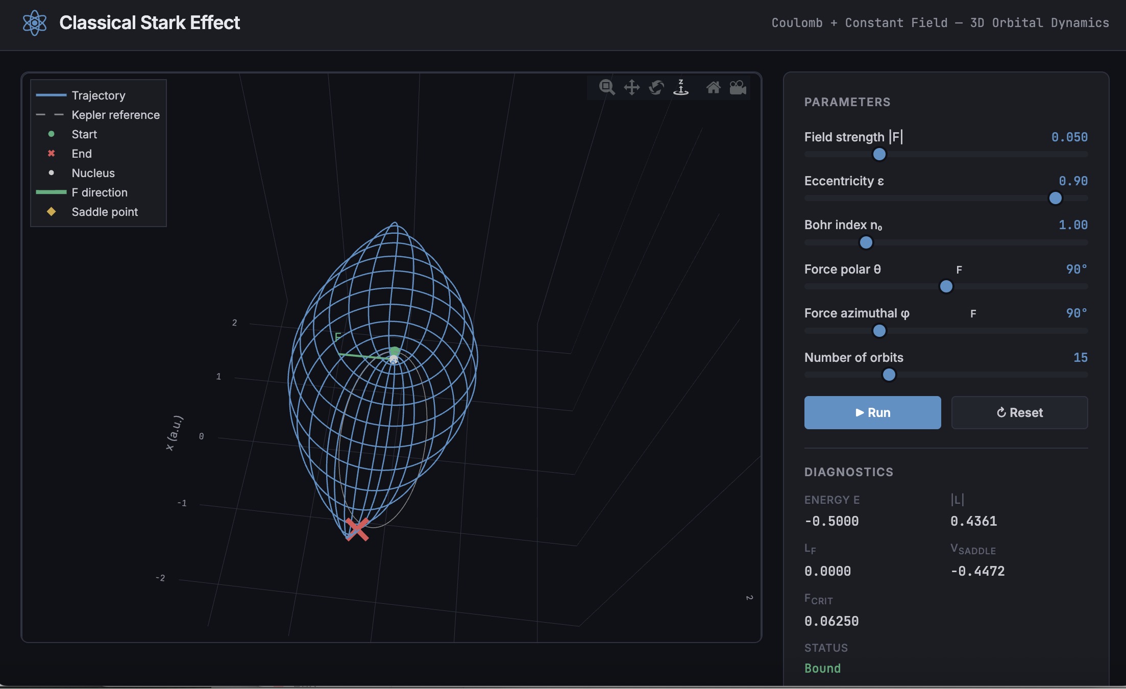
A Live Script can be converted to an HTML5 framework web application with AI as described in Double Pendulum Chaos Explorer: From HTML5 Prototype to MATLAB interactive application with AI. I have recently provides converted the Live Script Classical Stark Effect to a web application supporting a 3D twirlable display of motion of a particle subject to an inverse square law force plus an additional constant force - the problem known as the classical Stark effect.
The web application deployed to GitHub may be launched here and documents its dependencies below the interactive application. The files are available at Classical Stark Effect — Interactive Web Simulation. One gotcha was the need to enable hardware acceleration in Chrome (no problem in Safari) to support a 3D twirlable display. If hardware acceleration is disabled in Chrome, the application provides a warning and replaces the 3D twirlable display with a 2D alternate.
The conversion of the script to a web application was performed with Perplexity.ai. The GitHub deployment was accomplished with Anthropic's Claude using the open source GitHub CLI. WIth the gh CLI (already installed and authenticated on my Mac) via osascript, and Claude connected to my file system via MCP and an ngrok server, Claude executed on my Mac the following sequence of steps:
1. git init
Creates a hidden .git/ directory in the staging folder, initializing it as a local git repository. Before this command the folder is just a plain directory; after it, git can track files there. Run once per new project.
2. git branch -M main
Renames the default branch to main. Older git versions default to master; GitHub now expects main. The -M flag forces the rename even if main already exists. Must run after git init and before the first commit.
3. git add -A
Stages all files in the directory tree for the next commit. The -A flag means "all" -- new files, modified files, and deleted files are all included. This does not write anything to GitHub; it only updates git's internal index (the staging area) on your local machine.
4. git commit -m 'Initial release: Classical Stark Effect Interactive Simulation'
Takes everything in the staging area and freezes it into a permanent commit object stored in .git/. This is the snapshot that will be pushed. The -m flag provides the commit message inline. After this command, git knows exactly what files exist and what their contents are -- gh repo create --push will send exactly this snapshot.
5. gh repo create ClassicalStarkEffect --public --source=. --push
Three things happen in sequence inside this one command:
- gh repo create ClassicalStarkEffect --public -- calls the GitHub API to create a new empty public repository named ClassicalStarkEffect under the authenticated account (DuncanCarlsmith).
- --source=. -- tells gh to treat the current directory as the local git repo. It reads .git/ to find the commits and configures the remote.
- --push -- sets the new GitHub repo as origin and runs the equivalent of git push origin main, sending the commit from step 4 up to GitHub.
Without steps 1-4 having run first, --push would have nothing to send and the repo would land empty.
6. gh api repos/DuncanCarlsmith/ClassicalStarkEffect/pages --method POST -f build_type=legacy -f source[branch]=main -f 'source[path]=/'
Calls the GitHub REST API directly to enable GitHub Pages on the repo. Breaking down the flags:
- --method POST -- this is a create operation (not a read), so it uses HTTP POST.
- -f build_type=legacy -- critical flag. Tells GitHub to serve files directly from the branch. The alternative (workflow) would expect a .github/workflows/ Actions file to build and deploy the site, which doesn't exist here, and would produce a permanent 404.
- -f source[branch]=main -- serve from the main branch.
- -f 'source[path]=/' -- serve from the root of the branch (as opposed to a /docs subdirectory).
This is the API equivalent of going to Settings > Pages in the GitHub web UI and setting Branch: main, Folder: / (root), clicking Save.
7. curl -s -o /dev/null -w "%{http_code}" https://duncancarlsmith.github.io/ClassicalStarkEffect/
Not a git or gh command, but the verification step. GitHub Pages takes ~60 seconds to build after step 6. This curl fetches the live URL and prints only the HTTP status code (-w "%{http_code}"), discarding the body (-o /dev/null) and suppressing progress output (-s). 200 means live; 404 means still building.
An emirp is a prime that is prime when viewed in in both directions. They are not too difficult to find at a lower level. For example...
isprime([199 991])
Gosh, that was easy. But what happens if the number is a bit larger? The problem is, primes themselves tend to be rare on the number line when you get into thousands or tens of thousands of decimal digits. And recently, I read that a world record size prime had been found in this form. You have probably all heard of Matt Parker and numberphile.
And so, I decided that MATLAB would be capable of doing better. Why not? After all, at the time, the record size emirp had only 10002 decimal digits.
How would I solve this problem? First, we can very simply write a potential emirp as
10^n + a
then we can form the flipped version as
ahat*10^(n-d) + 1
where ahat is the decimally flipped version of a, and d is chosen based on the number of decimal digits in the number a itself. Not all emirps will be of that form of course, but using all of those powers of 10 makes it easy to construct a large number and its reversed form. And that is a huge benefit in this. For example,
Pfor = sym(10)^101 + 943
Prev = 349*sym(10)^99 + 1
It is easier to view these numbers using a little code I wrote, one that redacts most of those boring zeros.
emirpdisplay(Pfor)
emirpdisplay(Prev)
And yes, they are both prime, and they both have 102 decimal digits.
isprime([Pfor,Prev])
Sadly, even numbers that large are very small potatoes, at least in the world of large primes. So how do we solve for a much larger prime pair using MATLAB?
The first thing I want to do is to employ roughness at a high level. If a number is prime, then it is maximally rough. (I posted a few discussions about roughness some time ago.)
https://www.mathworks.com/matlabcentral/discussions/tips/879745-primes-and-rough-numbers-basic-ideas
In this case, I'm going to look for serious roughness, thus 2e9-rough numbers. Again, a number is k-rough if its smallest prime factor is greater than k. There are roughly 98 million primes below 2e9.
The general idea is to compute the remainders of 10^12345, modulo every prime in that set of primes below 2e9. This MUST be done using int64 or uint64 arithmetic, as doubles will start to fail you above
format short g
sqrt(flintmax)
The sqrt is in there because we will be multiplying numbers together here, and we need always to stay below intmax for the integer format you are working with. However, if we work in an integer format, we can get as high as 2e9 easily enough, by going to int64 or uint64.
sqrt(double(intmax('int64')))
And, yes, this means I could have gone as high as primes(3e9), however, I stopped at 2e9 due to the amount of RAM on my computer. 98 million primes seemed enough for this task. And even then, I found myself working with all of the cores on my computer. (Note that I found int64 arithmetic will only fire up the performance cores on your Mac via automatic multi-threading. Mine has 12 performance cores, even though it has 16 total cores.)
I computed the remainders of 10^12345 with respect to each prime in that set using a variation of the powermod algorithm. (Not powermod itself, which was itself not sufficiently fast for my purposes.) Once I had those 98 millin remainders in a vector, then it became easy to use a variation of the sieve of Eratosthenes to identify 2e9-rough numbers.
For example, working at 101 decimal digits, if I search for primes of the form 10^101+a, with a in the interval [1,10000], there are 256 numbers of that form which are 2e9-rough. Roughness is a HUGE benefit, since as you can see here, I would not want to test for primality all 10000 possible integers from that interval.
Next, I flip those 256 rough numbers into their mirror image form. Which members of that set are also rough in the mirror image form? We would then see this further reduces the set to only 34 candidates we need test for primality which were rough in both directions. With now only a few direct tests for primality, we would find that pair of 102 digit primes shown above.
Of course, I'm still needing to work with primes in the regime of 10000 plus decimal digits, and that means I need to be smarter about how I test a number to be prime. The isprime test given by sym/isprime only survives out to around 1000 decimal digits before it starts to get too slow. That means I need to perform Fermat tests to screen numbers for primality. If that indicates potential primality, I currently use a Miller-Rabin code to verify that result, one based on the tool Java.Math.BigInteger.isProbablePrime.
And since Wikipedia tells me the current world record known emirp was
117,954,861 * 10^11111 + 1 discovered by Mykola Kamenyuk
that tells me I need to look further out yet. I chose an exponent of 12345, so starting at 10^12345. Last night I set my Mac to work, with all cores a-fumbling, a-rumbling at the task as I slept. Around 4 am this morning, it found this number:
emirp = @(N,a) sym(10)^N + a;
Pfor = emirp(12345,10519197);
Prev = sym(flip(char(Pfor)));
emirpdisplay(Pfor)
emirpdisplay(Prev)
isProbablePrimeFLT([Pfor,Prev],210)
I'm afraid you will need to take my word for it that both also satisfy a more robust test of primality, as even a Miller-Rabin test that will take more time than the MATLAB version we get for use in a discussion will allow. As far as a better test in the form of the MATLAB isprime utility to verify true primality, that test is still running on my computer. I'll check back in a few hours to see if it fininshed.
Anyway, the above numbers now form the new world record known emirp pair, at 12346 decimal digits. Yes, I do recognize this is still what I would call low hanging fruit, that having announced a largest prime of this form, someone else willl find one yet larger in a few weeks or months. But even so, for the moment, MATLAB owns the world record!
If anyone else wants a version of the codes I used for the search, I've attached a version (emirpsearchpar.m) that employs the parallel processing toolbox. I do have as well a serial version which is of course, much, much slower. It would be fun to crowd source a larger world record yet from the MATLAB community.
Hey folks in MATLAB community! I'm an engineering student from India messing around with deep learning/ML for spotting faults in power electronics stuff—like inverter issues or microgrid glitches in Simulink.
What's your take?
- Which toolbox rocks for this—Deep Learning one or Predictive Maintenance?
- Any gotchas when training on sim data vs real hardware?
- Cool workflows or GitHub links you've used?
Would love your real experiences! 😊