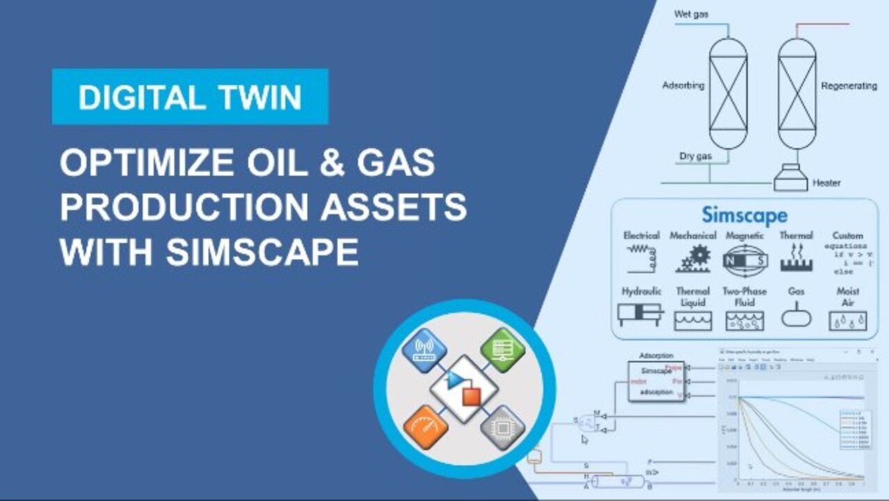
Optimize Oil & Gas Production Assets with Simscape

Design a digital twin for oil & gas production systems in Simscape and assemble physics-driven models for equipment components from prebuilt libraries to simulate and optimize production asset performance.

Highlights:

• Modeling a gas dehydration plant with process fluids (natural gas)
• Connecting Simulink and MATLAB with REFPROP for working with thermophysical properties of chemical components
• Calibrating the model to plant data to create digital twins for adsorption and absorption processes
• Modeling physics-driven systems