USB4 v2 SerDes Design & Signal Integrity Analysis with MATLAB - MATLAB
Video length is 31:09

USB4 v2 SerDes Design & Signal Integrity Analysis with MATLAB

Learn to design and analyze USB4 v2 systems using SerDes ToolboxTM and Signal Integrity ToolboxTM. In the rapidly evolving world of USB technology, the transition from NRZ to PAM3 modulation marks a significant leap forward for the next-generation USB standard, USB4 v2. This shift is driven by the demand for higher data rates and increased bandwidth, but it also introduces new challenges in SerDes design and signal integrity analysis.

Through this detailed walkthrough, viewers will gain insights into the complexities of creating a USB SerDes system that leverages PAM3 modulation to effectively manage transmitter and receiver equalization, addressing various forms of impairments such as jitter.

Starting with an introduction to the general SerDes and signal integrity workflow, the video demonstrates a hands-on approach to setting up a USB4 v2 SerDes model, beginning in the SerDes Designer app, progressing through detailed adjustments in Simulink®, and culminating in the analysis within the Signal Integrity Toolbox.

Through statistical and time-domain channel analysis, including the generation of IBIS-AMI models for SerDes and channel verification, the video provides a thorough understanding of the tools and techniques necessary for optimizing USB4 v2 systems.

Check out this example showing how to implement USB4 V2 (80Gbps PAM3) Transmitter and Receiver architectures with SerDes Designer and generate IBIS-AMI models using the library blocks in SerDes Toolbox: USB4 V2 Transmitter/Receiver IBIS-AMI Model

Recorded: 21 Jun 2023

Hello. My name is Andy Zambell. I'm a Senior Product Marketing Engineer at MathWorks. I've been at MathWorks for about two and a half years. Prior to joining MathWorks, I was a signal integrity engineer for about a decade where I developed high-speed connectors and cable assemblies. I was also involved in the development of industry standards such as IEEE 802.3 and OIF.

Today, I'll be covering SerDes design and Signal Integrity Analysis for USB4 2.0 IBUS-AMI models. Here's the agenda for today.

First, I'll start off by going over the general SerDes and Signal Integrity Workflow for MathWorks. Next, I'll show a demo of how to create a USB4 2.0 IBUS-AMI model where I'll start in the SerDes Designer app, move to Simulink to add more details to the model, and wrap up in Signal Integrity Toolbox for quick analysis. Then I'll summarize everything and I'll show you where to learn more.

A very brief overview of the SerDes and Signal Integrity Workflow goes as follows. Starting with SerDes' Toolbox, you can create IBUS-AMI models of a SerDes that can then be directly exported to Signal Integrity Toolbox. From there, you can perform pre-layout analysis of the system design. If there are any issues, you can move the entire system, stimulus, channel, and parameters back to SerDes Toolbox for debugging.

Another workflow that I won't talk about today, but will be the subject of a future webinar is post-layout verification with the RF PCB Toolbox. This workflow allows for the import of PCB schematics into Signal Integrity Toolbox to verify the design prior to building the PCB and for simulation to measurement correlation.

So on a high level, those are the typical workflows we have for the SerDes and signal integrity areas. Today, I'm going to show you a demo of how to create an IBUS-AMI model and use it in Signal Integrity Toolbox, so let's get started.

So here we are in the SerDes Designer app. Looking around the app, you can see in the upper-left here, we've got the configuration area. In the top middle here, we have the different types of blocks we can add, and for each block that we have here, we have different parameters for that block.

And then over here, we have Add Plots. So we can add a bunch of different types of plots, which will show up in this big empty area right here. So getting started for this USB4 2.0 IBUS-AMI model we want to set up, we'll start with the symbol time, which is 39.062 picoseconds, which corresponds to a data rate of 40 gigabits per second or baud rate of 25.6 gigabaud, since USB4 2.0 is a PAM3 modulation. So let's set the modulation to PAM3 real quick.

The samples per gigasymbol per the spec is 32. The differential signaling-- or, I'm sorry, the signaling is differentiable. And the target BER is 1.57e to the negative 8. Where does that come from? Again, it comes from the spec, but it comes from right here.

So this conversion factor is being used to go from the TER of 1e to the minus 8 to a BER of 1.57e to the minus 8. And the conversion factor is 11 bits over 7 trits. Again, this all comes directly from the standard.

OK. So the standard has a bunch of different equalization that we're going to add. So let's start adding some blocks. So we're going to add an FFE block to the transmitter. We're going to move over to the receiver and we're going to add two CTLE blocks with a two-stage CTLE. So we're going to add two blocks. And a DFE block.

So moving left to right, we'll start with the FFE. The FFE has two precursor taps and one postcursor tap. So four in total. The mode we're going to set to fixed, and normalize the taps as well. Move it over one block, the analog out, we're going to set the voltage to 0.4 volts and set the rise time to 7.8125 picoseconds, which is the 20 to 80% rise time of the symbol time.

The resistance is 42 and 1/2 ohms. It's an 85-ohm spec. And the capacitance isn't specified, so we're just going to use the default settings. Move over to the channel block. We're going to use a loss model. If we wanted to, we could import S parameters and use an impulse response of those S parameters, but we're just going to use a symbol loss model here.

We're going to set the channel loss to 9 and 1/2 dB. Again, this is the 85-ohm spec. And we'll set the target frequency to 12.8 gigahertz, which is the frequency of the baud rate. And move it over to the receiver, analog in. 42.5-ohm resistance, and we're going to use the default capacitance again.

OK. The CTLE. I'm going to add a 1 here and make it a little bit easier. And the mode. So we can choose the mode for the kettle. Adapt, all four fixed. We're going to have it adapt. The specification, you have your choice of combination of DC gain, AC gain, and peaking gain. But we are going to use a GPZ matrix.

I'll skip this gain pull zero matrix for just a second. Performance criteria. So how do you want the CTLE to adapt? What do you want it to maximize or minimize? We're going to set it to maximize the signal-to-noise ratio. And finally, the filter method, cascaded or partial fraction, we're going to use cascaded.

So this gain pull zero matrix, where is this coming from? We are actually going to use this MATLAB script here. This will calculate and create a variable for both matrices-- or, I'm sorry, for both CTLEs. It will have a matrix for each of the two CTLEs.

So up here is for the high-pull CTLE and down here is for the low-pull CTLE. So I'm going to run this and it'll create the two variables for me. Everything that you see in here was pulled out of the specification. So that's where all of these values come from. And as you can see, here's the two transfer functions for each of the two CTLEs.

Minimize these real quick. Come back to here. So we're on CTLE 1. And this would be GPZ, underscore, HP. And if I jump over here to the second CTLE, then, I can-- oops. CTLE 2. OK. So to adapt GPZ matrix, OK, this will be LP, loophole.

Now they're both set up, ready to go. Finally, the DFE. The DFE actually has 12 taps. So I'm just going to create eight more taps here. 8, 12. OK. OK, so the minimum and maximum tap values are set. Got 12 of them. Tap number one goes from 0 to 0.75. The rest of them, negative 0.2 to positive 0.2.

Get set to adapt. You have a choice of face detector. I'm going to use a bang-bang phase detector. So there we go. Everything is set up ready to go. I'm going to add a plot here. We're going to look at-- we'll look at the BER plot. Everything done in the SerDes Designer app is statistical. That's why everything's going to go fairly quickly.

The next step, when we move over to Simulink, we will look at time to main plots as well. So there's the DER. If I add a report as well, it'll give us the actual I measurements, height and width, as well it'll tell us what CTLE it used for each. It'll tell us what the DFE taps are. Just drag this over. You got them side by side. So there we go.

You can see the eye height, eye width area, things like that, two CTLEs that were used and our DFE taps that were used. Before we move on, I would like to add some jitter. So per the spec, I know we're going to use some random jitter and sinusoidal jitter in the TX. And we're going to use some random jitter in the RX.

So I'm going to turn all of those on. And this will save us a couple of seconds when we move over to Simulink. By checking these boxes, these reserve parameters will be added to the IBIS AMI model automatically. If we didn't have them checked, we could add them in Simulink if we wanted to.

So what are these values? I'm going to pull these right from the specification. Everything here is in unit interval. We could change the units if we wanted to. As you watch, every time I add some jitter, our =eye diagram is going to change.

I assume everything is going to be getting worse. So these jitter values are all the maximum values per the spec. So if you watch these numbers, they're all going down. You can see the I get a little bit smaller every time. And lastly, the random jitter of the receiver.

And there we go. So everything is set up and ready to go for us to go to Simulink. So I'm going to go up here to export, export SerDes system to Simulink. From here we're going to add some more detail with the jitter and with the FFE as well, as the CDR. Since there's no time domain in the SerDes Designer app, the CDR doesn't really do anything.

As we go to Simulink, we can add some settings for the CDR as we do our time domain plots there. OK, so here we are in Simulink. You can see we got a bunch of blocks here. So just kind of going around Simulink. Open up the configuration block. And the configuration block has carried over everything from the configuration area in SerDes Designer app.

So you can see the symbol time is the same, samples per symbol, things like that. OK, jumping down here to the stimulus. So this is where we set the stimulus for our simulation. We're going to increase this to 50,000 symbols.

Waveform creation method, so we're going to use a serial PRBS waveform. And we need to change the mapping, the binary to pan am mapping. Luckily, we have this all set up, ready to go for USB4. So that's all done. Hit OK.

So the transmitter bearing down near the transmitter. You can see the FFE. So that's that. Jumping back up, our analog channel. Again, everything from our channel was carried over, loss model, loss, impedance, things like that. All of our analog in and out models were also here.

We want to look at the channel responses real quick. Impulse response, step response, pulse response, that's all there. If you change your mind and you want to import an S parameter, you can do so. You just click this button. And a window will open up that will allow you to import a touchstone file.

So this one's just pointing to a default touchstone file. So you would just browse to your touchstone file and import it from here. But again, we're just going to continue to stick with the loss model we have.

And finally, going into the receiver, we see our two CTLEs and our DFEs. So looking at our one CTLE, you can see that the GPZ matrix that the variable was also carried along. Visualize the response, so we can look at this transfer function.

And if we compare the two, they look identical. So that's good. Close everything. And in the DFE, make this bigger, again, all of our taps, tap settings, things like that carried along. The CDR, so now that we're going to be doing time domain simulations, we're going to set the CDR sensitivity to five millivolts. Everything else we're just going to leave alone.

So there we go. That's set up and ready to go. OK, one thing that needs to change for our transmitter in the FFE is we need to set a bunch of values. So the spec has something like 40 some odd preset FFE settings. And we want to import them all to be able to use them in this IBIS AMI model.

So to do that, we need to go to configuration and open SerDes IBIS AMI manager. There we go, opens. Before we do that real quick, let's just take a look at this IBIS AMI manager.

So when we go to export it, you get your choice of what it is you want to export. So in this case, it's a transmitter receiver. Change the name of the actual IBIS models. We'll just call this my USB TX. Let's call it 4. And again, my USB4 RX.

The corner percentage we'll leave the default at 10%. So what type of AMI models do we want to export? We're going to do dual models instead of just get wave only or init only. Number of bits to ignore, since it's a four tap FFE, we'll do four taps. We will increase this to the number of bits to ignore to I'll say 30,000 bits.

So we ignore the first 30,000 bits. We're simulating 50,000. We'll ignore the first 30,000 of them. And real quick, we'll set this to changes to my USB4 as well. So there we go. So that's all set, ready to go.

A quick preview of the IBIS portion of the model right here. OK, so we want to set up the FFE. So how do we do that? In the TX, we have the FFE here. We want to add a parameter. So we click on the FFE, click Add Parameter.

Then we're going to give it a name and a description here. So new parameter name, we're going to call this config select. And we're going to give it a description of transmitter FFE presets. So there's that. Leave the usage as in, the type as integer. And the format we'll change to list.

I'm just going to put the default as zero. So the list values and the list tip values, I'm going to copy them over here. So we stretch this out, make sure everything looks correct. Yell at me if I have something incorrect.

So as you can see, there's a total of 43 different settings for the FFE. So these are their values and just basically names here. So hit OK. So there we go. So all we did there was to add placeholders for the different tap settings. We didn't actually add the tap settings quite yet.

So that's what we're going to do next. So I'm going to go back up here to the TX, go into the init block, hit refresh. I'm going to hit show init. So what we're going to do is add those preset FFE settings for the statistical portion of the IBIS AMI model. And then we're going to do the same thing for the time domain portion of the IBIS AMI model.

So how do we do this? We are going to scroll down a little bit. And in this section right down here is where we add our own custom user code, which I have over here. And I will paste it in. So there you go. You can see all the different cases with all of these different preset FFE tap settings that again, all come directly from the standard.

So now that this is done, we're going to move over and add the settings for the time domain portion of the IBIS AMI model. So to do this, I'm going to go back to the TX. I'm going to control view on the FFE to kind of go deeper into it. And you can see that here's the config select parameter that we added.

So what we're going to do is we're going to add a MATLAB function block, which comes out of the library browser, Simulink, user defined functions, and MATLAB functions. So we're going to add that over here. Close the browser. Zoom out a bunch so I can see everything.

OK, move this out of the way. Open up the MATLAB function block. And here we're going to add a function. In this function I have over here, I'm going to paste it in. It's going to look similar to what I added earlier for the statistical vert portion of the IBIS AMI model.

So there we go. That's added. We can go back to here. Makes this a little bit bigger. OK, I'll need to delete that one. Bring this over to here. All right, so now I just need to reconnect everything.

And finally, there we go. So we have the tap weights and the config select coming into our function block here. Tap weights coming out into the FFE. So that's all good to go now. Go back up and back up. So now that we've done everything we needed to do for the FFE, we can now set up the jitter.

To do that, we will go back into the configuration block, back into the SerDes IBIS AMI model manager and go to each of the jitter settings. You want to click on the transmitter random jitter and click Edit. And what we're going to do here is we're going to set it up so we can have a range of values.

I'll just quickly copy this. And format range. We'll have it default to zero. The minimum value is zero. And the maximum value's there. Add zero to the current value as well. So that's one down, two to go. The other two are going to be done the exact same way.

OK, now everything's set up. Jitter's done. Feed forward equalizer is all set and ready to go. We are ready to simulate. So I'm going to come up here and hit Run. As it's running, it's first going to initialize everything. And an I diagram will pop up. So you can see the I diagram live as the simulation is running. So I hit Run. We can watch it.

So now that the simulation is done, we can take a look at some of these results. Make this a little bit bigger, easier to see. So you can see it plots the pulse response, and the waveform, statistical I, and another report. And then down here at the bottom is the time domain I and the time domain metrics.

And you may observe a difference between the statistical and time domain waveforms. In the time domain stimulation, the effects of symbol encoding to control ISI and also real time DFE behavior may contribute to improved performance. Conversely, statistical simulation utilizes frequency domain convolution rather than symbol by symbol stimulus. It does not include the effects of symbol encoding or signal conditioning by DFE.

So now that we've looked at our results, we can now export everything to signal integrity toolbox. First, we're going to go to Configuration, open SerDes IBIS AMI manager, so we can export the IBIS AMI models to use in signal integrity toolbox. So I already set all this up. All I got to do is hit Export.

We can then use the models in signal integrity toolbox. OK, so now that we've exported the IBIS AMI model, close, open up signal integrity link so we can export this IBIS AMI model to signal integrity toolbox.

So we'll give it a name, my USB4. All we got to do is click the button, Create Serial Link Project. After a few seconds, you see it gives you a log file. It just tells you what exactly it did. Hit Close. And now that's all done, you can see that it creates a project for us. It puts the TX and the RX right in the middle of our schematic here. And it just puts a lossy transmission line in here as well.

So what we're going to do real quick is I'm just going to run a simulation. I'm going to set the traces to vary from two, four, six, and eight inches. So I can run a quick simulation. So we're going to see if everything works correctly, just to make sure our IBIS AMI models are functioning as we expect them to.

I set everything up, set the trace lengths with the two to eight inches. I'm going to hit the Simulate button up there. Save it. I'm going to run everything in parallel. I have four cores on my CPU. And I'm going to run four simulations. I'm basically just going to run one pass. Hit Run, wait a couple of minutes till it's done.

So now that the simulation is done running, let's take a look at some results. So the results that we're going to look at, they're going to be in the Signal Integrity Viewer app. If you look down here at the bottom, we have three tabs, Network, Statistical, and Time Domain. So let's plot real quick some insertion loss plots.

So I'm going to grab all four of these, right click, S parameters and DB, insertion loss differential. We're going to take a quick look at all of these. OK, nothing terribly exciting. It's just some varying trace lengths. So let's take a look at the statistical BER plot. So I'm going to add a new display real quick.

Now we're going to look at one show BER. So for this to pop up to see if we've got an open I. And we do. So there you go. So that's the statistical BER plot. And now we'll look at the time domain persistent I.

The other thing you can do instead of right clicking display or to add a new display, you can just check this box to create a new one every time you plot something. So now we'll just look at the persistent BER, so the time domain eye diagram. So there's that. So you can see got three tabs down here.

We can look at various things. And like I said, nice, wide open eye diagrams. So it looks like this IBIS AMI model's performing as expected. If we had any issues, we could come back and export it back into Simulink. We just come here, click the Import Serial Link Project. So I'm actually going to hit refresh first.

And it just updates to our project here in the Signal Integrity Toolbox, check off what we want to send back to Simulink. And then you just click the Import Serial Link Project. And then you can address any issues in Simulink that may have arisen in Signal Integrity Toolbox.

So in summary, we started off in SerDes designer app to lay the groundwork for the USB4 V2 IBIS AMI model. Then we move the model to Simulink, where we were able to fine tune the model for jitter and feedforward equalization. Then we moved to Signal Integrity Toolbox, where we use the IBIS AMI model on a simple channel just to make sure it works as intended.

And had there been any issues with the model, we could bring everything back into Simulink to address any problems there. If you want to learn more about SerDes and signal integrity solutions for MathWorks, you can look over the SerDes and Signal Integrity product and documentation pages for both of those toolboxes and try the various examples there.

You check out the IBIS AMI discovery page to learn more about the ins and outs of IBIS AMI models. And finally, you can check out the videos page and watch the SerDes and Signal Integrity videos there. Thank you very much. In just a minute we'll start the Q&A portion of the webinar.

View more related videos