hornScrimp
Create Scrimp horn antenna
Description
The default hornScrimp object creates a Scrimp horn antenna
resonating around 3.91 GHz. Scrimp (short circular ring loaded horn with minimized
cross-polarization) horn antenna is a short, axially corrugated horn antenna with a single
slot. Using this antenna provides high aperture efficiency, low cross-polarization, and low
voltage standing wave ratio (VSWR) over a broad frequency band. These antennas are used for
navigation satellite feeder links in a medium earth orbit (MEO).

Creation
Description
ant = hornScrimp
ant = hornScrimp(PropertyName=Value)PropertyName is the property
name and Value is the corresponding value. You can specify several
name-value arguments in any order as
PropertyName1=Value1,...,PropertyNameN=ValueN. Properties that you
do not specify, retain their default values.
For example, hornScrimp(ConeHeight=0.05) creates Scrimp horn
antenna with a cone height of 0.05 meters.
Properties
Object Functions
axialRatio | Calculate and plot axial ratio of antenna or array |
bandwidth | Calculate and plot absolute bandwidth of antenna or array |
beamwidth | Beamwidth of antenna |
charge | Charge distribution on antenna or array surface |
current | Current distribution on antenna or array surface |
design | Create antenna, array, or AI-based antenna resonating at specified frequency |
efficiency | Calculate and plot radiation efficiency of antenna or array |
EHfields | Electric and magnetic fields of antennas or embedded electric and magnetic fields of antenna element in arrays |
feedCurrent | Calculate current at feed for antenna or array |
impedance | Calculate and plot input impedance of antenna or scan impedance of array |
info | Display information about antenna, array, or platform |
memoryEstimate | Estimate memory required to solve antenna or array mesh |
mesh | Generate and view mesh for antennas, arrays, and custom shapes |
meshconfig | Change meshing mode of antenna, array, custom antenna, custom array, or custom geometry |
msiwrite | Write antenna or array analysis data to MSI planet file |
optimize | Optimize antenna and array catalog elements using SADEA or TR-SADEA algorithm |
pattern | Plot radiation pattern of antenna, array, or embedded element of array |
patternAzimuth | Azimuth plane radiation pattern of antenna or array |
patternElevation | Elevation plane radiation pattern of antenna or array |
peakRadiation | Calculate and mark maximum radiation points of antenna or array on radiation pattern |
rcs | Calculate and plot monostatic and bistatic radar cross section (RCS) of platform, antenna, or array |
resonantFrequency | Calculate and plot resonant frequency of antenna |
returnLoss | Calculate and plot return loss of antenna or scan return loss of array |
show | Display antenna, array, AI-based antenna, platform, or shape |
sparameters | Calculate S-parameters for antenna or array |
stlwrite | Write mesh information to STL file |
vswr | Calculate and plot voltage standing wave ratio (VSWR) of antenna or array element |
Examples
Create Scrimp horn antenna with default properties.
ant = hornScrimp
ant =
  hornScrimp with properties:

             Radius: 0.0292
    WaveguideHeight: 0.0250
         FeedHeight: 0.0175
          FeedWidth: 3.0000e-04
         FeedOffset: 0.0200
         ConeHeight: 0.0362
         ConeRadius: 0.0408
     ApertureRadius: 0.0480
     ApertureHeight: 0.0250
         StubHeight: 0.0146
          Conductor: [1×1 metal]
               Tilt: 0
           TiltAxis: [1 0 0]
               Load: [1×1 lumpedElement]
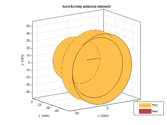
View the antenna using the show function.
show(ant)
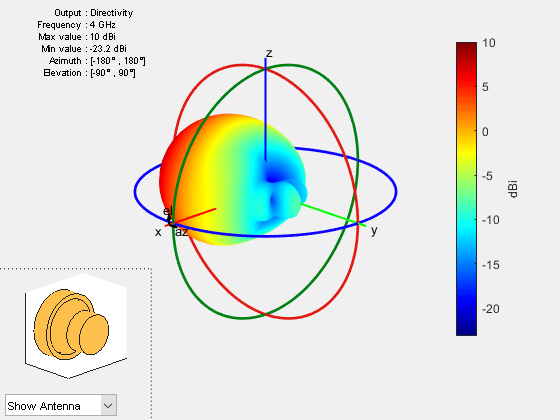
Plot the radiation pattern of the Scrimp horn antenna at a frequency of 4 GHz.
pattern(ant,4e9)
Create Scrimp horn antenna with the aperture radius of 0.06 meters.
ant = hornScrimp;
ant.ApertureRadius = 0.06;
Visualize the antenna using the show function.
show(ant)

Plot the S-parameters over a frequency range of 3.6 GHz to 4.5 GHz.
s = sparameters(ant,linspace(3.6e9,4.5e9,51));
rfplot(s)

More About
References
[1] Muhammad, S. A., A. Rolland, S. H. Dahlan, R. Sauleau, and H. Legay. “Hexagonal-Shaped Broadband Compact Scrimp Horn Antenna for Operation in C-Band.” IEEE Antennas and Wireless Propagation Letters 11 (2012): 842–45.
[2] Muhammad, S., A. Rolland, S. H. Dahlan, R. Sauleau and H. Legay. “Comparison Between Scrimp Horns and Stacked Fabry-Perot Cavity Antennas with Small Apertures.” 2012 6th European Conference on Antennas and Propagation (EUCAP) (2012): 817–820.
Version History
Introduced in R2021a