monopoleCustom
Create customized monopole antenna
Description
The default monopoleCustom object creates a monopole radiator
of any shape using the antenna.Shape class resonating around 1.24 GHz. The
ground plane can take any shape. You can create any arbitrarily shaped monopole and analyze it
for field, surface, and port characteristics. Monopole antennas have a simple structure and
provide omnidirectional radiation patterns with wide impedance bandwidth. Monopole antennas
are commonly used in airborne and ground-based communication systems.

Creation
Description
ant = monopoleCustom
ant = monopoleCustom(PropertyName=Value)PropertyName is the property
name and Value is the corresponding value. You can specify several
name-value arguments in any order as
PropertyName1=Value1,...,PropertyNameN=ValueN. Properties that you
do not specify, retain their default values.
For example, ant = monopoleCustom(RadiatorTilt=90) creates a
monopole antenna with tilt angle of the radiator at 90 degrees on the
z-axis.
Properties
Object Functions
axialRatio | Calculate and plot axial ratio of antenna or array |
bandwidth | Calculate and plot absolute bandwidth of antenna or array |
beamwidth | Beamwidth of antenna |
charge | Charge distribution on antenna or array surface |
current | Current distribution on antenna or array surface |
efficiency | Calculate and plot radiation efficiency of antenna or array |
EHfields | Electric and magnetic fields of antennas or embedded electric and magnetic fields of antenna element in arrays |
feedCurrent | Calculate current at feed for antenna or array |
impedance | Calculate and plot input impedance of antenna or scan impedance of array |
info | Display information about antenna, array, or platform |
memoryEstimate | Estimate memory required to solve antenna or array mesh |
mesh | Generate and view mesh for antennas, arrays, and custom shapes |
meshconfig | Change meshing mode of antenna, array, custom antenna, custom array, or custom geometry |
msiwrite | Write antenna or array analysis data to MSI planet file |
optimize | Optimize antenna and array catalog elements using SADEA or TR-SADEA algorithm |
pattern | Display antenna radiation pattern in Site Viewer |
patternAzimuth | Azimuth plane radiation pattern of antenna or array |
patternElevation | Elevation plane radiation pattern of antenna or array |
peakRadiation | Calculate and mark maximum radiation points of antenna or array on radiation pattern |
rcs | Calculate and plot monostatic and bistatic radar cross section (RCS) of platform, antenna, or array |
resonantFrequency | Calculate and plot resonant frequency of antenna |
returnLoss | Calculate and plot return loss of antenna or scan return loss of array |
show | Display antenna, array, AI-based antenna, platform, or shape |
sparameters | Calculate S-parameters for antenna or array |
stlwrite | Write mesh information to STL file |
vswr | Calculate and plot voltage standing wave ratio (VSWR) of antenna or array element |
Examples
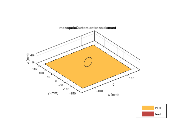
Create a disc monopole with a of radius 25 mm, on a square ground plane of 30 cm, and with a feed gap of 0.7 mm.
Rad = antenna.Circle(Radius=25e-3);
FeedStrip = antenna.Rectangle(Length=1e-3,Width=0.7e-3,...
    Center=[0 -(Rad.Radius+(0.7e-3)*0.3)]);
m = monopoleCustom;
m.Radiator = Rad + FeedStrip;
m.GroundPlane = antenna.Rectangle(Length=300e-3,Width=300e-3);
View the antenna using the show function.
show(m)
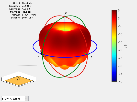
Plot the radiation pattern of the antenna at 2.05 GHz.
p = PatternPlotOptions(MagnitudeScale=[-40 5]);
pattern(m,2.05e9,PatternOptions=p);
References
[1] Ammann, M. J. “Square Planar Monopole Antenna.” IEE National Conference on Antennas and Propagation, vol. 1999, IEE, pp. 37–40.
[2] Weiner, M. “Monopole Element at the Center of a Circular Ground Plane Whose Radius Is Small or Comparable to a Wavelength.” IEEE Transactions on Antennas and Propagation, vol. 35, no. 5, pp. 488–495.
[3] N. P. Agrawall, G. Kumar and K. P. Ray, "Wide-band planar monopole antennas," in IEEE Transactions on Antennas and Propagation, vol. 46, no. 2, pp. 294-295.
Version History
Introduced in R2020b