Create Low-Order LPV Model of CPU and Heat Sink Model

Since R2024a

Step 3 of 4 in Thermal Modeling and Control Design for CPU Chip Cooling System

This example shows you how to obtain a low-order linear parameter-varying (LPV) surrogate for the high-fidelity finite element model of the heat sink. This is an alternative to the modal approximation of the used in the previous step of the tutorial. In this example, you focus on preserving the input/output response of the finite element model implemented in the CPU + HeatSink block in the ChipCoolingSystem Simulink® model while drastically reducing the complexity and simulation time.

Because the fan speed determines mass flow rate $$\underset{}{\overset{\dot{}}{m}}$$ which impacts the convection coefficient, the CPU + HeatSink dynamics are nonlinear of this form.

$$E\underset{}{\overset{\dot{}}{x}}=A(\underset{}{\overset{\dot{}}{m}})x+BQ+f(\underset{}{\overset{\dot{}}{m}})T_{\infty }$$

$$T=Cx$$

Here, $$x$$ is the temperature distribution, $$Q$$ the heat generated by the CPU, $$T$$ the socket temperature, and $$T_{\infty }$$ the ambient temperature. This makes LPV model a natural choice for this application.

Initialization and Parameters

Open the project file.

prj = openProject("CPUChipCoolingControl");

To create the finite element model and extract the data for use with Descriptor State Space block, run the initialization scripts provided with the project.

heat_sink_defs
fan_defs
sensor_defs
clear sys
sys.A = (Q+K); % multiply by -1 in DSS block
sys.B = speye(nDoF,nDoF);
sys.C = speye(nDoF,nDoF);
sys.D = sparse(nDoF,nDoF);
sys.E = M;
Tinf = 294;  % ambient temp

Batch Linearization

This example provides a Simulink model for linearization with predefined linear analysis input and output points.

open_system("HeatSinkLinearize")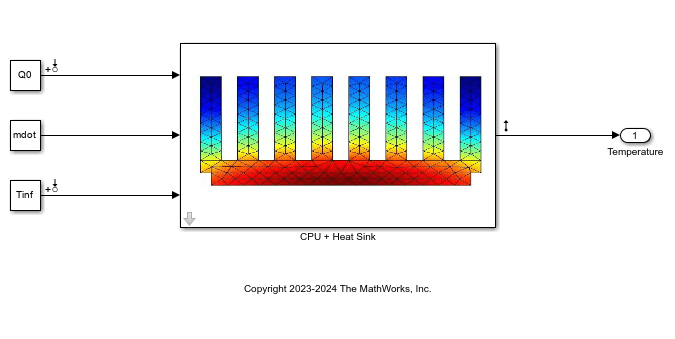

Here, you obtain sparse linearized models of the CPU + HeatSink block for seven values of mass flow rate $$\underset{}{\overset{\dot{}}{m}}$$. Perform linearization at a uniform temperature of 323 K, which is the operating temperature of the CPU at full capacity. Since the model is linear in $$Q$$, the generated heat is set to zero.

Define the parameters.

Q0 = 0;
IC = 323;   
N = 7;
mdotValues = linspace(0.005,0.025,7);  
mdot = 0.005;

Linearizing this model requires high memory allocation. Therefore, before you run the simulation, consider closing any other applications with high memory requirements.

Perform a batch linearization for the seven $$\underset{}{\overset{\dot{}}{m}}$$ values.

linio = getlinio("HeatSinkLinearize");
param = struct("Name","mdot","Value",mdotValues);
tic
spsys = linearize("HeatSinkLinearize",linio,param);
toc

Elapsed time is 115.218440 seconds.

size(spsys)

7x1 array of sparse state-space models.
Each model has 1 outputs, 2 inputs, and 30362 states.

spsys is a 7-by-1 array of sparse state-space models, each with 30362 states due to the feedback loops which are represented in differential algebraic equation (DAE) form.

Plot the frequency response. The inputs are the heat source $$Q$$ and ambient temperature $$T_{\infty }$$. This plot shows how mass air flow (fan speed) affects both the gain and time constant of the heat removal characteristics.

w = logspace(-6,1,100);
fsys = frd(spsys,w);
bode(fsys)
grid on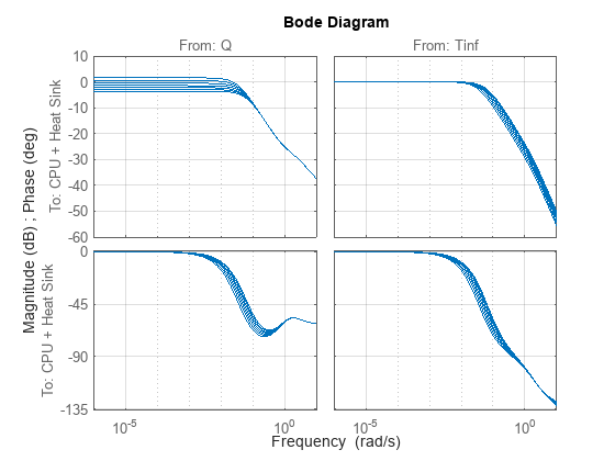

Model Order Reduction

The model order reduction tools available in Control System Toolbox™ software cannot reduce an array of sparse models in a state-consistent way. To circumvent this limitation, reduce the midrange model and apply the projectors $$V,W$$ to the other models. Use sparse balanced Truncation to reduce the model for the midrange $$\underset{}{\overset{\dot{}}{m}}$$ value.

Create a model order specification object using the reducespec function.

spsysREF = spsys(:,:,4);
R = reducespec(spsysREF,"balanced");
R = process(R);

Initializing...
Running ADI with built-in shifts........
Solved Lyapunov equations to desired accuracy.

Plot the bar chart of Hankel singular values and associated error bounds.

view(R)

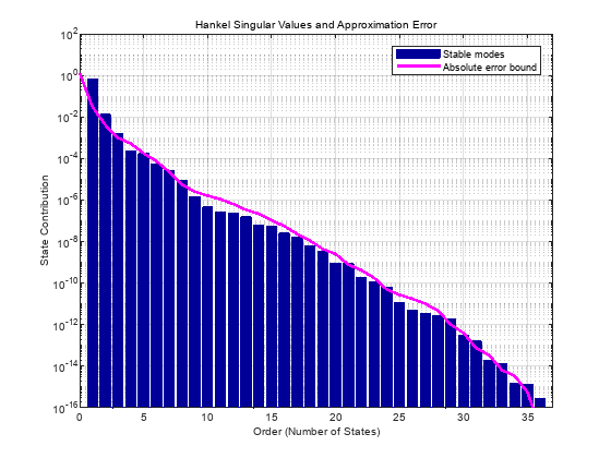
The singular value chart suggests you need fewer than 10 states for high accuracy. For this model, choose an order of five.

[rsysREF,info] = getrom(R,Order=5,Method="truncate");

Compare the response of full-order and reduced-order models.

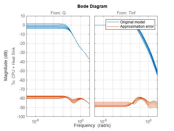
fsysREF = fsys(:,:,4);
sigma(fsysREF,fsysREF-rsysREF)
grid on
legend("Original model","Approximation error",Location="best")

A plot of the approximation error relative to the original model confirms an error of less than 0.01% at DC.

Now apply the same projectors $$V,W$$ to the other models to obtain a reduced-order model for each $$\underset{}{\overset{\dot{}}{m}}$$ value.

W = info.PL;  
V = info.PR;
clear ssarray
for ct=1:N
   [A,B,C,D,E] = sparssdata(spsys(:,:,ct));
   ssarray(:,:,ct) = dss(W'*A*V,W'*B,C*V,full(D),W'*E*V);
end
ssarray.InputName = spsys.InputName;
ssarray.SamplingGrid = struct("mdot",mdotValues);

This approach is not guaranteed to work in general, but here it does a good job for all $$\underset{}{\overset{\dot{}}{m}}$$ values and all I/O pairs. This figure shows low approximation error for all models in the array.

bodemag(fsys,fsys-ssarray)
grid on
legend("Original model","Approximation error")

LPV Model

So far you have obtained fifth-order models that closely match the input/output response of the full-order 30362 state linearizations for seven values of mass air flow. Now you can use the LPV System block to interpolate the dynamics as a function of $$\underset{}{\overset{\dot{}}{m}}$$ to approximate the nonlinear behavior of the CPU + HeatSink block in Simulink®.

To prepare for this, eliminate the $\mathit{E}$ matrix from the state-space array.

ssarray = ss(ssarray,"explicit");

Also eliminate the $$T_{\infty }$$ input by turning it into a derivative offset and attaching it to the state-space models. This step is optional, and you can just keep $$T_{\infty }$$ as an input to all models.

Offsets = struct("dx",cell(N,1));
for ct=1:N
   [~,B] = ssdata(ssarray,ct);
   Offsets(ct).dx = B(:,2)*Tinf;
end
ssarray.Offsets = Offsets;
ssarray = ssarray(:,1);
size(ssarray)

7x1 array of state-space models.
Each model has 1 outputs, 1 inputs, and 5 states.

The model now contains just the heat source as an input.

Simulink Comparison

Use the Simulink models HeatSinkPDE and HeatSinkLPV to compare the full-order model and its LPV approximation for a scenario where you inject a constant heat source $$Q=20$$, ramp up the fan to full speed, and then ramp it down.

Initialize the simulation from steady state with uniform temperature equal to the ambient temperature $$T_{\infty }$$ and compute a matching initial condition for the reduced-order models with zero heat source and ambient temperature using the findop function.

op = findop(ssarray(:,:,1),y=Tinf,u=0)

op = 
  OperatingPoint with properties:

            x: [5×1 double]
            u: 0
            w: [0×1 double]
           dx: [5×1 double]
            y: 294
           rx: [5×1 double]
           ry: -0.0180
    Equations: 6
     Unknowns: 5
       Status: 'Overconstrained problem, residuals may exist. Returned least-squares solution.'

x0r = op.x;

The full-order model HeatSinkPDE simulation takes over 36 hours to complete, therefore this example provides the simulation results in the simResults.mat file.

Simulate the LPV model.

IC = Tinf;  % reset IC to original value
open_system("HeatSinkLPV");

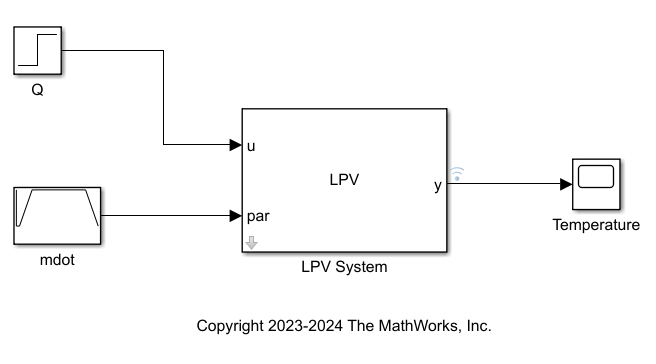
simOut = sim("HeatSinkLPV");
lpvsim = simOut.logsout{1}.Values;

LPV simulation runs under 5 seconds.

Compare the simulation results.

load simResults fullsim
figure
plot(fullsim.Time,fullsim.Data,lpvsim.Time,lpvsim.Data,"r--")
grid on
legend("Full-order simulation (30+ hours)",...
        "LPV simulation (under 5 seconds)",Location="best")

The LPV model provides an accurate approximation of the full-order model, and the simulation results are indistinguishable.