Import Finite Element Model Data to Simulink

Since R2024a

Step 2 of 4 in Thermal Modeling and Control Design for CPU Chip Cooling System

This example shows how to use the data generated from a model created using Partial Differential Equation Toolbox™ software to simulate a finite element (FE) model in Simulink®. In this example, you also apply a model order reduction technique to the finite element model to speed up the simulation by reducing the number of degrees of freedom to compute.

System Overview

The system in this Simulink® model is a variable-speed fan cooling a CPU which, depending on the model and its operating point, can generate variable amount of heat. Each component of the system is modeled using empirical data and technical specifications. The CPU + HeatSink model allows you to choose two levels of modeling fidelity: a full-order FE model and a reduced-order model. The full-order FE model accurately captures all the thermal dynamics; however this is not necessary for model-based design iterations. Using a reduced-order model, the software only needs to calculate the dynamics associated with the frequency range of interest.

Open the model.

prj = openProject("CPUChipCoolingControl");
mdl = "ChipCoolingSystem";
open_system(mdl)

Control Loop Components

CPU and Heat Sink Plant

The plant in this system is the thermal dynamics of a heat-generating CPU and a heat-dissipating heat sink modeled as a finite element model. The FE matrices generated form a system of ordinary differential equations that you can solve using the Descriptor State-Space (Simulink) block. Run the script heat_sink_defs to create the model and extract FE matrices.

heat_sink_defs
pdeplot3D(heatsink.Geometry.Mesh)

Define the input matrices for the Descriptor State-Space block.

sys.A = (Q+K); % multiply by -1 in DSS block
sys.B = speye(nDoF,nDoF);
sys.C = speye(nDoF,nDoF);
sys.D = sparse(nDoF,nDoF);
sys.E = M;
sys.IC = IC*ones(nDoF,1);
sys.femodel = heatsink;

Actuation

In this model, you approximate the performance of the cooling fan using numbers in the typical range of consumer grade fans. The two values of interest for the fan are the RPM output from an input voltage and the corresponding volumetric flow rate at that RPM. For simplicity, this example provides maximum values for RPM and CFM, and linearly interpolated intermediate values depending on the voltage and RPM inputs. Additionally, this example uses:

• The fan performance data obtained using fan performance plots from manufacturers and digitized into a data table using the plot digitization tool GRABIT [1]. Using this plot digitization to lookup table technique, the model captures nonlinearities better by adding more data points.

• The mass flow rate data obtained from the International Standard Atmosphere model. You can use the atmosisa (Aerospace Toolbox) function to get an air density of 1.2250 kg/m^3 at sea level.

• Inertial effects introduced to the fan model to account for the delay from voltage input to RPM output. You can obtain such data from the Thermistor-Controlled Fan (Simscape Electrical) example by running the DC motor with a rotational inertia of $1\times {10}^{-5}$ kg$\times$m^2 attached to it at 12V and computing the time to reach 63.2% of the steady state rotational velocity. Then, use this value as a first-order time constant.

You can also add additional requirements for noise levels to test whether or not a specific fan model is capable of adequately cooling a CPU while staying sufficiently quiet for customer requirements.

Load the fan data and plot the results.

fan_defs
plot(V2CFM(:,1),V2CFM(:,2)); 
xlabel("Volts"); 
ylabel("CFM")

Sensor

The sensor temperature dynamics, like the fan inertial effects, are modeled by a first-order time constant. For this example, chip-level thermal behavior is typically in the order of one second, so use a value of one second. The time constant is specific to each sensor depending on the type of sensor and the application. Typically, the manufacturer of the sensor provides this information. The value may also be a function of another variable, in which case you can apply the plot digitization workflow again. As discussed in the following section, the compensation is based on case temperature, so this is where the sensor is located.

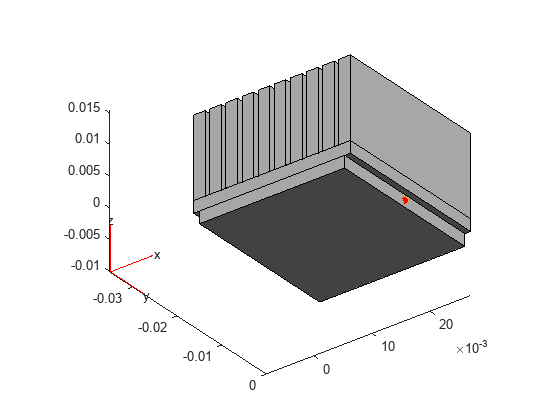
Load the sensor data and plot the results. The script heat_sink_defs defines the sensor location which is shown as a red dot in following figure.

sensor_defs
pdegplot(heatsink)
view([37.5 -30])
hold on
scatter3(m.Nodes(1,outID),m.Nodes(2,outID),...
         m.Nodes(3,outID),"MarkerFaceColor",[1 0 0])

Compensation

To enforce a temperature limit of 70.0°C on the processor case, the model uses a PI controller. Typically, the manufacturer provides the temperature limits that you can easily integrate into this model. To avoid overheating, the temperature limit setpoint for the controller is specified as 50.0°C. A 12 V electric motor drives the cooling fan in this model. The controller output is saturated to a lower limit of 0 V, indicating the motor is not running and there is no forced convective cooling, and an upper limit of 12 V, which corresponds to the highest speed of the motor and, therefore, the highest convective heat transfer the system is capable of.

Model Order Reduction

The finite element formulation of the heat equation on the heat sink is computationally intensive and requires matrix equations of size 18664-by-18664. The size of this system is too large to be practical for model-based design workflows. Therefore, you can use a reduced-order model (ROM) to approximate the dynamics and speed up simulation time. This example uses a projection technique to perform modal truncation described by these equations.

$${\mathit{A}}_{\mathit{r}}={\mathit{V}}^{\mathit{T}}\mathit{AV}$$

$${\mathit{B}}_{\mathit{r}}={\mathit{V}}^{\mathit{T}}\mathit{B}$$

$${\mathit{C}}_{\mathit{r}}=\mathit{CV}$$

$${\mathit{D}}_{\mathit{r}}=\mathit{D}$$

$${\mathit{E}}_{\mathit{r}}={\mathit{V}}^{\mathit{T}}\mathrm{EV}$$

Use the modalTruncation function provided with this example to obtain the ROM formulation. To construct a ROM, this function solves the original model in the specified frequency range and uses the reduce (Partial Differential Equation Toolbox) function. For this system, restrict the ROM to retain only the modes with frequencies that lie within the range of 0 to 10 rad/s.

freqRange = [0 10];
rsys = modalTruncation(sys,freqRange);

Running the Model

You can now simulate the model and determine the effectiveness of the control system. Using a SimulinkInput object and parsim, run 100 heat loading simulations.

nSims = 100;
in(1:nSims) = Simulink.SimulationInput(mdl);
for i = 1:nSims
    in(i) = setBlockParameter(in(i),[mdl+"/Heat Generation"], ...
                                "ActiveScenario", ['Scenario' num2str(i)]);
end
out = parsim(in,"TransferBaseWorkspaceVariables","on");

[12-Jan-2024 09:57:57] Checking for availability of parallel pool...
[12-Jan-2024 09:57:57] Starting Simulink on parallel workers...
[12-Jan-2024 09:57:59] Loading project on parallel workers...
[12-Jan-2024 09:57:59] Configuring simulation cache folder on parallel workers...
[12-Jan-2024 09:57:59] Transferring base workspace variables used in the model to parallel workers...
[12-Jan-2024 09:57:59] Loading model on parallel workers...
[12-Jan-2024 09:58:05] Running simulations...
[12-Jan-2024 09:58:13] Completed 1 of 100 simulation runs
[12-Jan-2024 09:58:13] Completed 2 of 100 simulation runs
[12-Jan-2024 09:58:14] Completed 3 of 100 simulation runs
[12-Jan-2024 09:58:16] Completed 4 of 100 simulation runs
[12-Jan-2024 09:58:20] Completed 5 of 100 simulation runs
[12-Jan-2024 09:58:20] Completed 6 of 100 simulation runs
[12-Jan-2024 09:58:22] Completed 7 of 100 simulation runs
[12-Jan-2024 09:58:26] Completed 8 of 100 simulation runs
[12-Jan-2024 09:58:26] Completed 9 of 100 simulation runs
[12-Jan-2024 09:58:26] Completed 10 of 100 simulation runs
[12-Jan-2024 09:58:26] Completed 11 of 100 simulation runs
[12-Jan-2024 09:58:26] Completed 12 of 100 simulation runs
[12-Jan-2024 09:58:27] Completed 13 of 100 simulation runs
[12-Jan-2024 09:58:28] Completed 14 of 100 simulation runs
[12-Jan-2024 09:58:32] Completed 15 of 100 simulation runs
[12-Jan-2024 09:58:33] Completed 16 of 100 simulation runs
[12-Jan-2024 09:58:33] Completed 17 of 100 simulation runs
[12-Jan-2024 09:58:36] Completed 18 of 100 simulation runs
[12-Jan-2024 09:58:40] Completed 19 of 100 simulation runs
[12-Jan-2024 09:58:40] Completed 20 of 100 simulation runs
[12-Jan-2024 09:58:40] Completed 21 of 100 simulation runs
[12-Jan-2024 09:58:40] Completed 22 of 100 simulation runs
[12-Jan-2024 09:58:40] Completed 23 of 100 simulation runs
[12-Jan-2024 09:58:40] Completed 24 of 100 simulation runs
[12-Jan-2024 09:58:45] Completed 25 of 100 simulation runs
[12-Jan-2024 09:58:46] Completed 26 of 100 simulation runs
[12-Jan-2024 09:58:46] Completed 27 of 100 simulation runs
[12-Jan-2024 09:58:48] Completed 28 of 100 simulation runs
[12-Jan-2024 09:58:53] Completed 29 of 100 simulation runs
[12-Jan-2024 09:58:53] Completed 30 of 100 simulation runs
[12-Jan-2024 09:58:53] Completed 31 of 100 simulation runs
[12-Jan-2024 09:58:53] Completed 32 of 100 simulation runs
[12-Jan-2024 09:58:53] Completed 33 of 100 simulation runs
[12-Jan-2024 09:58:53] Completed 34 of 100 simulation runs
[12-Jan-2024 09:58:58] Completed 35 of 100 simulation runs
[12-Jan-2024 09:58:59] Completed 36 of 100 simulation runs
[12-Jan-2024 09:58:59] Completed 37 of 100 simulation runs
[12-Jan-2024 09:59:01] Completed 38 of 100 simulation runs
[12-Jan-2024 09:59:06] Completed 39 of 100 simulation runs
[12-Jan-2024 09:59:06] Completed 40 of 100 simulation runs
[12-Jan-2024 09:59:06] Completed 41 of 100 simulation runs
[12-Jan-2024 09:59:06] Completed 42 of 100 simulation runs
[12-Jan-2024 09:59:06] Completed 43 of 100 simulation runs
[12-Jan-2024 09:59:06] Completed 44 of 100 simulation runs
[12-Jan-2024 09:59:11] Completed 45 of 100 simulation runs
[12-Jan-2024 09:59:12] Completed 46 of 100 simulation runs
[12-Jan-2024 09:59:12] Completed 47 of 100 simulation runs
[12-Jan-2024 09:59:14] Completed 48 of 100 simulation runs
[12-Jan-2024 09:59:19] Completed 49 of 100 simulation runs
[12-Jan-2024 09:59:19] Completed 50 of 100 simulation runs
[12-Jan-2024 09:59:19] Completed 51 of 100 simulation runs
[12-Jan-2024 09:59:19] Completed 52 of 100 simulation runs
[12-Jan-2024 09:59:19] Completed 53 of 100 simulation runs
[12-Jan-2024 09:59:19] Completed 54 of 100 simulation runs
[12-Jan-2024 09:59:23] Completed 55 of 100 simulation runs
[12-Jan-2024 09:59:24] Completed 56 of 100 simulation runs
[12-Jan-2024 09:59:24] Completed 57 of 100 simulation runs
[12-Jan-2024 09:59:26] Completed 58 of 100 simulation runs
[12-Jan-2024 09:59:31] Completed 59 of 100 simulation runs
[12-Jan-2024 09:59:31] Completed 60 of 100 simulation runs
[12-Jan-2024 09:59:31] Completed 61 of 100 simulation runs
[12-Jan-2024 09:59:31] Completed 62 of 100 simulation runs
[12-Jan-2024 09:59:31] Completed 63 of 100 simulation runs
[12-Jan-2024 09:59:32] Completed 64 of 100 simulation runs
[12-Jan-2024 09:59:35] Completed 65 of 100 simulation runs
[12-Jan-2024 09:59:36] Completed 66 of 100 simulation runs
[12-Jan-2024 09:59:36] Completed 67 of 100 simulation runs
[12-Jan-2024 09:59:40] Completed 68 of 100 simulation runs
[12-Jan-2024 09:59:43] Completed 69 of 100 simulation runs
[12-Jan-2024 09:59:43] Completed 70 of 100 simulation runs
[12-Jan-2024 09:59:43] Completed 71 of 100 simulation runs
[12-Jan-2024 09:59:43] Completed 72 of 100 simulation runs
[12-Jan-2024 09:59:43] Completed 73 of 100 simulation runs
[12-Jan-2024 09:59:43] Completed 74 of 100 simulation runs
[12-Jan-2024 09:59:49] Completed 75 of 100 simulation runs
[12-Jan-2024 09:59:49] Completed 76 of 100 simulation runs
[12-Jan-2024 09:59:49] Completed 77 of 100 simulation runs
[12-Jan-2024 09:59:51] Completed 78 of 100 simulation runs
[12-Jan-2024 09:59:56] Completed 79 of 100 simulation runs
[12-Jan-2024 09:59:56] Completed 80 of 100 simulation runs
[12-Jan-2024 09:59:56] Completed 81 of 100 simulation runs
[12-Jan-2024 09:59:56] Completed 82 of 100 simulation runs
[12-Jan-2024 09:59:56] Completed 83 of 100 simulation runs
[12-Jan-2024 09:59:56] Completed 84 of 100 simulation runs
[12-Jan-2024 10:00:02] Completed 85 of 100 simulation runs
[12-Jan-2024 10:00:02] Completed 86 of 100 simulation runs
[12-Jan-2024 10:00:02] Completed 87 of 100 simulation runs
[12-Jan-2024 10:00:05] Completed 88 of 100 simulation runs
[12-Jan-2024 10:00:09] Completed 89 of 100 simulation runs
[12-Jan-2024 10:00:09] Completed 90 of 100 simulation runs
[12-Jan-2024 10:00:09] Completed 91 of 100 simulation runs
[12-Jan-2024 10:00:09] Completed 92 of 100 simulation runs
[12-Jan-2024 10:00:09] Completed 93 of 100 simulation runs
[12-Jan-2024 10:00:10] Completed 94 of 100 simulation runs
[12-Jan-2024 10:00:16] Completed 95 of 100 simulation runs
[12-Jan-2024 10:00:16] Completed 96 of 100 simulation runs
[12-Jan-2024 10:00:16] Completed 97 of 100 simulation runs
[12-Jan-2024 10:00:19] Completed 98 of 100 simulation runs
[12-Jan-2024 10:00:22] Completed 99 of 100 simulation runs
[12-Jan-2024 10:00:22] Completed 100 of 100 simulation runs
[12-Jan-2024 10:00:22] Cleaning up parallel workers...

You can use the Simulation Manager to plot the signals of interest and compare the simulations. Running the simulations using the reduced order model, allows you to analyze many loading scenarios rapidly. To open Simulation Manager, run the following command.

openSimulationManager(in,out)

Upon completion, you can visualize the socket temperature and verify that the chip does not overheat, therefore validating the system design.

References

[1] Jiro Doke (2024). GRABIT (https://www.mathworks.com/matlabcentral/fileexchange/7173-grabit), MATLAB Central File Exchange.