Tune PI Controller for Heat Sink Model

Since R2024a

Step 4 of 4 in Thermal Modeling and Control Design for CPU Chip Cooling System

This example shows how to tune a PI controller to drive the cooling fan and control the temperature of the heat sink model. In this example, you use the LPV model created in the previous step of the tutorial to tune the controller.

Open the project.

prj = openProject("CPUChipCoolingControl");

Run the initialization scripts for heat sink, fan, and sensor data.

fan_defs;
sensor_defs;
heat_sink_defs;
IC = 323;

Control Architecture

You can try simple PI control to drive the fan and keep the temperature at or below the 50 C (323.15 K) limit. Here, you use positive feedback so that the error is positive when this limit exceeds, and negative otherwise. Using positive PI gains applies a positive voltage to the fan when the limit temperature exceeds. The PI Controller block output in this model is set to saturate outside of the range 0 to 12 Volts. This means that the controller applies a zero voltage when the temperature is below the limit and no corrective action is needed. In other words, the controller only acts on positive error to remove heat and does nothing for negative error.

This example implements the architecture in the PIDControlCL Simulink® model. Open the model.

open_system('PIDControlCL')

Plant Models

To use available tools for PID tuning, first obtain models of the plant seen by the PI controller, which includes the Cooling Fan, CPU + HeatSink, and Sensor blocks. Here, the plant is nonlinear with dynamics depending on voltage which drives the fan speed and mass air flow. To obtain low-order plant models for several voltage settings between 0 to 12 volts, you can leverage the surrogate LPV model obtained in the previous step. For convenience, use the open-loop model PIDControlOL with generated heat $$Q$$ and voltage $$V$$ as inputs, and socket temperature $$T$$ as output. The LPV model data is provided in the model workspace.

open_system('PIDControlOL')

Pick five voltage values in the operating range:

V = linspace(2,10,5);

When linearizing this model, you must carefully pick the operating conditions based on physics. Since the fan kicks in only above 323 K and is meant to prevent the CPU temperature to rise much above this value, the controller operates mostly around $$T=323K$$. For each voltage $$V$$, use findop (Simulink Control Design) to compute the heat amount $$Q$$ for which the CPU+HeatSink model reaches an equilibrium temperature of 323 K.

opt = findopOptions(DisplayReport='off');
opspec = operspec('PIDControlOL',size(V));
for ct=1:numel(V)
   % Set input voltage
   opspec(ct).Inputs(2).Known = 1;
   opspec(ct).Inputs(2).u = V(ct);
   % Set operating temperature
   opspec(ct).Outputs(1).Known = 1;
   opspec(ct).Outputs(1).y = 323;   
   % Determine heat Q for equilibrium
   opspec(ct).Inputs(1).Known = 0;
end
[op,report] = findop('PIDControlOL',opspec,opt);

Now that you have equilibrium conditions op for each voltage level, linearize the model around each of these conditions to obtain the local linear plant dynamics.

G = linearize('PIDControlOL',op);
G.SamplingGrid = struct('V',V);
G.InputName = {'Q';'V'};
G.OutputName = 'T';

bode(G)
grid on

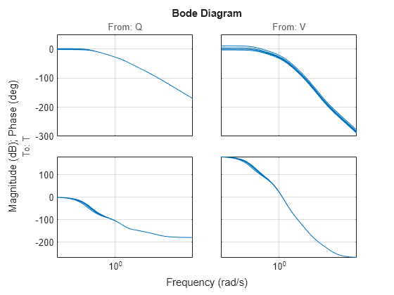
The Bode plot shows variability similar to that observed for the ssarray models of the CPU + HeatSink block. Note that phase is consistent with the action of each input: temperature increases with $$Q$$ (zero phase at DC) and decreases with voltage (180 degrees phase at DC).

PI Tuning

Control System Toolbox software provides several PID tuning techniques, including automated tuning with pidTuner or PID Tuner, multimodel tuning with systune, and gain-scheduled PID design using either one. In this example, you use pidtune to tune the controller on the second plant ($$V=4$$) with a target response time of about 5 seconds. Since the main goal is to compensate the effect of $$Q$$, use a pidtuneOptions object to set the emphasis on disturbance rejection. Finally, use a minus sign with the plant input to pidtune to account for use of positive feedback in control architecture.

Defined the options and tune the controller.

opt = pidtuneOptions('DesignFocus','disturbance-rejection','PhaseMargin',45);
C = pidtune(-G(:,'V',2),'pi',1/5,opt)

C =
 
             1 
  Kp + Ki * ---
             s 

  with Kp = 2.18, Ki = 0.383
 
Continuous-time PI controller in parallel form.

Simulate the linear response to a step disturbance in heat $$Q$$.

C.InputName = 'T';
C.OutputName = 'V';
CL = connect(G,C,'Q','T');
step(CL)

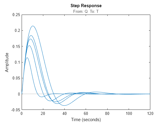
These responses are satisfactory so move the gains P = 2.18 and I = 0.383 to the PID block for nonlinear validation. Simulate the model to a heat step of 30 maintained for 200 seconds.

set_param('PIDControlCL/PID Controller','P','2.18','I','0.383')
simOut1 = sim('PIDControlCL');
plot(simOut1.logsout{1}.Values.Time,simOut1.logsout{1}.Values.Data)
grid on
title("Socket Temperature")
xlabel("Time (s)")
ylabel("Temperature (K)")

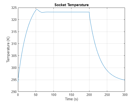
The fan turns on above 323K and keeps the temperature near this value until the heat source subsides.

Anti-Windup

As mentioned earlier, the voltage is constrained to the range $$[0,12]$$ and the controller can only act on positive error (it can only remove heat). Whenever you combine integral action with a saturation, there is potential for integrator windup, which is the accumulation of error while the controller output is saturated. Such accumulation takes time to unwind, causing delayed reaction and sometimes instability. Here, for example, a PI controller normally accumulates negative error while temperature is below the limit and the applied voltage is zero. When the temperature finally exceeds the limit, it can take a long time for the integrator to flush this accumulated negative error and finally issue a positive voltage command. To prevent this, configure the PID block to use clamping anti-windup, which essentially stops integration when saturating. To see what happens without anti-windup, set the anti-windup selection to none and run the simulation.

set_param('PIDControlCL/PID Controller','AntiWindupMode','none')
simOutAW = sim('PIDControlCL');
plot(simOutAW.logsout{1}.Values.Time,simOutAW.logsout{1}.Values.Data)
grid on
title("Socket Temperature")
xlabel("Time (s)")
ylabel("Temperature (K)")

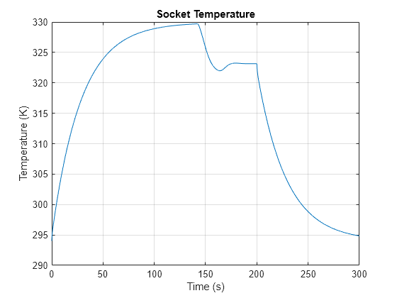
The controller response is now severely lagging, allowing the temperature to rise to unacceptable values. This delayed reaction is due to the build-up of negative error in the integrator up to the time when socket temperature reaches its limit, and the error becomes positive.

Proportional Gain

Proportional action is also important when operating near saturation. To see this, zero out the proportional term and run the simulation.

set_param('PIDControlCL/PID Controller','AntiWindupMode','clamping','P','0')
simOutP0 = sim('PIDControlCL');
plot(simOutP0.logsout{1}.Values.Time,simOutP0.logsout{1}.Values.Data)
grid on
title("Socket Temperature")
xlabel("Time (s)")
ylabel("Temperature (K)")

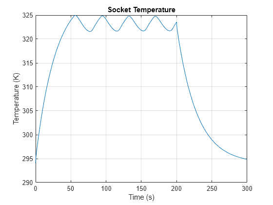
The response now has a limit cycle with the temperature oscillating around the limit value. Despite anti-windup, the integrator still lags enough to never quite catch up with error sign changes.

vSim = simOutP0.logsout{2}.Values;
errSim = simOutP0.logsout{3}.Values;
plot(vSim.Time,vSim.Data,errSim.Time,errSim.Data)
legend("Command voltage","Error")
grid on
xlabel("Time (s)")

Proportional action mitigates this by reducing lag. In fact, you can improve the response by increasing the proportional gain suggested by pidtune. For example, increase the gain value to 3.

set_param('PIDControlCL/PID Controller','AntiWindupMode','clamping','P','3')
simOutP = sim('PIDControlCL');
plot(simOutP.logsout{1}.Values.Time,simOutP.logsout{1}.Values.Data)
grid on
title("Socket Temperature")
xlabel("Time (s)")
ylabel("Temperature (K)")

vSimP = simOutP.logsout{2}.Values;
errSimP = simOutP.logsout{3}.Values;
plot(vSimP.Time,vSimP.Data,errSimP.Time,errSimP.Data)
legend("Command voltage","Error",Location="best")
grid on
xlabel("Time (s)")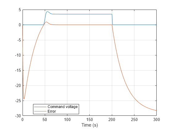

Close the models.

close_system('PIDControlOL',0)
close_system('PIDControlCL',0)

The LPV surrogate model allows you to run the simulations for several design scenarios quickly. You can now run the full-fidelity finite element model with the desired control specification.