Create Heat Sink Finite Element Model and Export Data for State-Space Simulation

Since R2024a

Step 1 of 4 in Thermal Modeling and Control Design for CPU Chip Cooling System

This example shows how to convert a finite element (FE) model to a form that you can easily use in a Simulink® model for a closed-loop control system. For this example, the plant model is the thermal dynamics of a heat-generating CPU with a heat-dissipating heat sink. Using Partial Differential Equation Toolbox™ software, you can model these dynamics using a finite element formulation of the heat equation on a 3-D geometry. You can then generate the finite element matrices which you can solve using the Descriptor State Space block for simulation in Simulink®.

Open the project.

prj = openProject("CPUChipCoolingControl");

Construct Heat Sink Finite Element Model

For this heat sink model, define the width W, fin height H, fin thickness t, and the number of fins nFin.

W = 27*10^-3;
H = 17.5*10^-3;
t = 2*10^-3;
nFin = 10;

Call the geometry utility function createHeatSinkGeometry to return a geometry object for the FE model. This function is provided with this example and takes in the heat sink width, fin height, fin thickness, and the number of fins as inputs and creates a DiscreteGeometry object. The function creates a 2D geometry and extrudes it to a distance equal to the width, thus the depth and width have the same value. The function also returns the face numbers of the internal faces of the fins in a vector forcedBCfaces. These faces will have the fan induced airflow from the cooling fan along them. The freeBCfaces output contains the remaining faces.

[gm,forcedBCfaces,freeBCfaces] = createHeatSinkGeometry(W,H,t,nFin);

Define the geometry and problem type of the FE model.

heatsink = femodel(AnalysisType="ThermalTransient", ...
                   Geometry=gm);

Define the minimum edge length and growth rate for the mesh, and create a mesh node location for the temperature sensor placement in the heat sink casing.

heatsink = generateMesh(heatsink,Hmin=t,Hgrad=1.9); % try to min(nDoF)
m = heatsink.Geometry.Mesh;
CPUcell = 1;
outID = findNodes(m,"nearest",[0.026 -W/2 -t/2]'); % middle of yz side of casing

Define the internal properties of the heat sink material to complete the construction of the heat sink model.

k = 210; % W*m^-1*K^-1
rho = 2710; % kg/m^3
Cp = 900; % J*kg^-1*K^-1
heatsink.MaterialProperties = ...
    materialProperties(ThermalConductivity=k, ...
                       MassDensity=rho, ...
                       SpecificHeat=Cp); % aluminum alloy 6060 T6

Visualize the model.

pdeplot3D(m)

Model Heat Transfer

Specify an internal heat load representing the heat generation from a CPU. You use this heat load as an input to the DSS block in Simulink in the next step.

chipHeat = 1; % Watts
chipW = 25e-3; % m
chipL = W; % m
chipH = t; % m
heatPerVol = chipHeat/(chipL*chipW*chipH); % W/m^3
heatsink.CellLoad(CPUcell) = cellLoad(Heat=heatPerVol);
IC = 294; % Kelvin
heatsink.CellIC = cellIC(Temperature=IC);

The dominant mode of heat transfer in this scenario is due to convection and is governed by this equation.

$$\dot{\mathit{q}}=\mathit{h}\left({\mathit{T}}_{\infty }-\mathit{T}\right)$$

The coefficient $\mathit{h}$ is the convective heat transfer coefficient. It varies as a function of mass flow rate and is determined experimentally. For simplicity, this example uses values interpolated linearly between a free convection coefficient (no airflow) to a maximum forced convection coefficient.

To construct a lookup table for a mass flow dependent coefficient value, use empirically derived values provided in hCoeffData.txt. This dependency is approximately linear, so it is modeled using the Gain and Bias blocks in the provided HeatSinkSubsys model.

Tinf = IC; % ambient temperature, Kelvin
rho = 1.225; % kg/m^3
h_free = 9.0;
h_forced = [ 0.0, h_free; ...
             readmatrix("hCoeffData.txt")];
p = polyfit(h_forced(:,1),h_forced(:,2),1);
h_gain = p(1); 
h_bias = p(2);

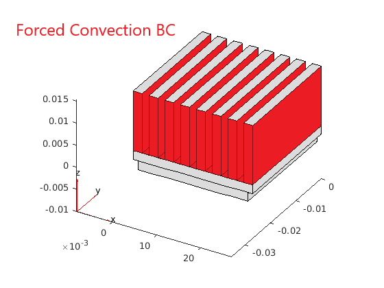
Construct a convective boundary condition for the ducted airflow where you apply forced convection coefficients on the internal fin surfaces that see airflow, and free convection coefficients on the external facing surfaces of the system.

heatsink.FaceLoad(freeBCfaces) = faceLoad(Heat=1); % used as convective BC
heatsink.FaceLoad(forcedBCfaces) = faceLoad(Heat=1); % used as convective BC

Construct Simulink System

Generate the finite element formulation matrices. For more information about these matrices, see assembleFEMatrices (Partial Differential Equation Toolbox).

femat = assembleFEMatrices(heatsink);
K = femat.K; 
M = femat.M; 
A = femat.A; 
F = femat.F; 
Q = femat.Q;
G = femat.G;
H = femat.H;
R = femat.R;

Finally, construct the vectors used in Simulink to apply the heat generation, forced convection, and free convection.

nDoF = size(K,1);
freeBCnodes = findNodes(m,"Region","Face",freeBCfaces);
unitFreeBC = zeros(nDoF,1);
unitFreeBC(freeBCnodes) = 1;
normalizedFreeBC = zeros(nDoF,1);
normalizedFreeBC(freeBCnodes) = G(freeBCnodes);
forcedBCnodes = findNodes(m,"Region","Face",forcedBCfaces);
unitForcedBC = zeros(nDoF,1);
unitForcedBC(forcedBCnodes) = 1;
normalizedForcedBC = zeros(nDoF,1);
normalizedForcedBC(forcedBCnodes) = G(forcedBCnodes);
x0 = ones(nDoF,1)*IC;
unitCPUHeat = full(F);

This example provides the HeatSinkSubsys model which implements the CPU heat generation and heat sink convective heat transfer model.