cassegrainOffset
Create offset Cassegrain antenna
Description
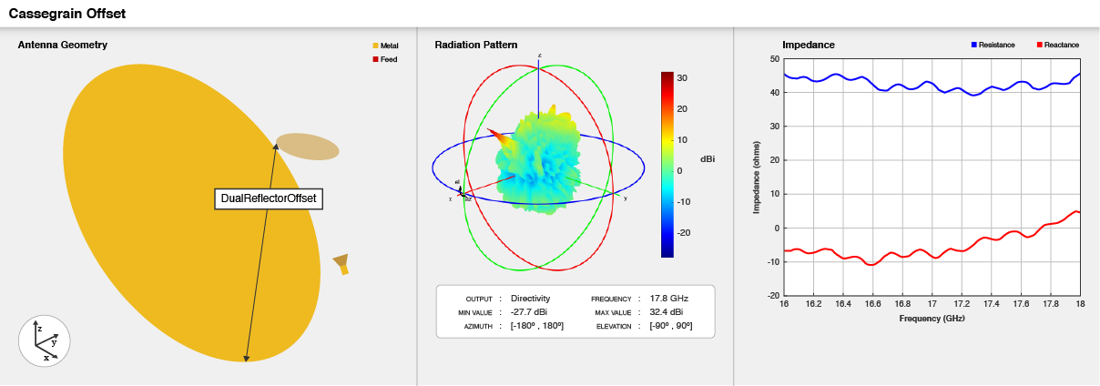
The default cassegrainOffset object creates an offset
Cassegrain antenna resonating around 17.8 GHz. The offset Cassegrain antenna is a parabolic
antenna, where the feed antenna is mounted off-axis to convex sub reflector and concave main
reflector. The asymmetric arrangement of reflectors provides less blockage for waves
redirected from main reflector. The advantage of these antennas is high gain, reduced
sidelobes and improved cross polarization. The offset Cassegrain antennas are used in
satellite communication ground antennas, radar systems, and, radio telescopes among other
applications.
Creation
Description
ant = cassegrainOffset
ant = cassegrainOffset(PropertyName=Value)PropertyName is the property
name and Value is the corresponding value. You can specify several
name-value arguments in any order as
PropertyName1=Value1,...,PropertyNameN=ValueN. Properties that you
do not specify, retain their default values.
For example, ant = cassegrainOffset(FocalLength=0.04) creates an
offset Cassegrain antenna with the focal length of the main reflector set to 40
mm.
Properties
Object Functions
axialRatio | Calculate and plot axial ratio of antenna or array |
bandwidth | Calculate and plot absolute bandwidth of antenna or array |
beamwidth | Beamwidth of antenna |
charge | Charge distribution on antenna or array surface |
current | Current distribution on antenna or array surface |
design | Create antenna, array, or AI-based antenna resonating at specified frequency |
efficiency | Calculate and plot radiation efficiency of antenna or array |
EHfields | Electric and magnetic fields of antennas or embedded electric and magnetic fields of antenna element in arrays |
feedCurrent | Calculate current at feed for antenna or array |
impedance | Calculate and plot input impedance of antenna or scan impedance of array |
info | Display information about antenna, array, or platform |
memoryEstimate | Estimate memory required to solve antenna or array mesh |
mesh | Generate and view mesh for antennas, arrays, and custom shapes |
meshconfig | Change meshing mode of antenna, array, custom antenna, custom array, or custom geometry |
msiwrite | Write antenna or array analysis data to MSI planet file |
optimize | Optimize antenna and array catalog elements using SADEA or TR-SADEA algorithm |
pattern | Plot radiation pattern of antenna, array, or embedded element of array |
patternAzimuth | Azimuth plane radiation pattern of antenna or array |
patternElevation | Elevation plane radiation pattern of antenna or array |
peakRadiation | Calculate and mark maximum radiation points of antenna or array on radiation pattern |
rcs | Calculate and plot monostatic and bistatic radar cross section (RCS) of platform, antenna, or array |
resonantFrequency | Calculate and plot resonant frequency of antenna |
returnLoss | Calculate and plot return loss of antenna or scan return loss of array |
show | Display antenna, array, AI-based antenna, platform, or shape |
solver | Specify FMM and FEM solver settings during electromagnetic analysis |
sparameters | Calculate S-parameters for antenna or array |
stlwrite | Write mesh information to STL file |
vswr | Calculate and plot voltage standing wave ratio (VSWR) of antenna or array element |
Examples
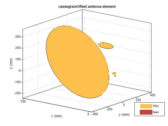
Create an offset Cassegrain dual-reflector antenna with default properties.
ant = cassegrainOffset
ant =
  cassegrainOffset with properties:

                 Exciter: [1×1 hornConical]
                  Radius: [0.3475 0.0650]
             FocalLength: 0.5000
     MainReflectorOffset: 0.5000
         InterAxialAngle: 5
    DualReflectorSpacing: 0.0350
           ReflectorTilt: [53.1300 11.3700]
                    Tilt: 0
                TiltAxis: [1 0 0]
                    Load: [1×1 lumpedElement]
              SolverType: 'MoM-PO'
View the antenna using the show function.
show(ant)
Plot the radiation pattern of offset Cassegrain dual-reflector antenna at a frequency of 18 GHz.
pattern(ant,18e9)

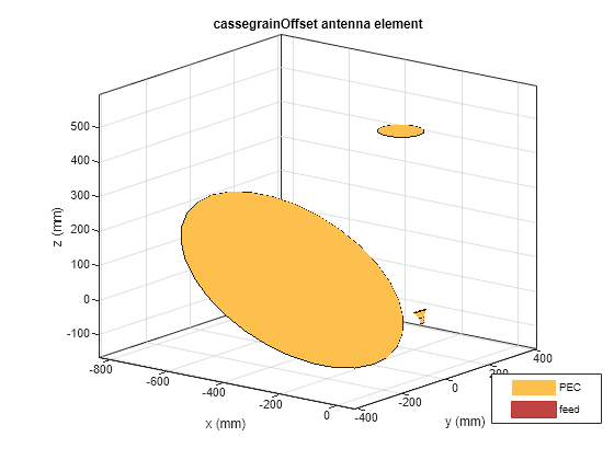
Create and view offset Cassegrain antenna with optimum reflector tilt angles and with a focal length of 0.8 meters and an interaxial angle of 5 degrees.
ant = cassegrainOffset(InterAxialAngle=5,FocalLength=0.8)
ant =
  cassegrainOffset with properties:

                 Exciter: [1×1 hornConical]
                  Radius: [0.3475 0.0650]
             FocalLength: 0.8000
     MainReflectorOffset: 0.5000
         InterAxialAngle: 5
    DualReflectorSpacing: 0.0350
           ReflectorTilt: [53.1300 11.3700]
                    Tilt: 0
                TiltAxis: [1 0 0]
                    Load: [1×1 lumpedElement]
              SolverType: 'MoM-PO'
View the antenna using the show function.
show(ant)

View offset cassegrain antenna with optimum reflector tilt angles.
ant.ReflectorTilt = ant.BasisReflectorTilt
ant =
  cassegrainOffset with properties:

                 Exciter: [1×1 hornConical]
                  Radius: [0.3475 0.0650]
             FocalLength: 0.8000
     MainReflectorOffset: 0.5000
         InterAxialAngle: 5
    DualReflectorSpacing: 0.0350
           ReflectorTilt: [34.7080 0.9748]
                    Tilt: 0
                TiltAxis: [1 0 0]
                    Load: [1×1 lumpedElement]
              SolverType: 'MoM-PO'
View the antenna using the show function.
show(ant)
Calculate the impedance of the antenna over a frequency span 17 GHz - 18 GHz.
impedance(ant,linspace(17e9,18e9,27))

Create a linear array of bowtie antennas.
e = bowtieTriangular(Tilt=90,TiltAxis=[0 1 0]);
arr = linearArray(Element=e, ElementSpacing=0.25);
Create an offset Cassegrain antenna with the linear array as the exciter.
ant = cassegrainOffset(Exciter=arr)
ant =
  cassegrainOffset with properties:

                 Exciter: [1×1 linearArray]
                  Radius: [0.3475 0.0650]
             FocalLength: 0.5000
     MainReflectorOffset: 0.5000
         InterAxialAngle: 5
    DualReflectorSpacing: 0.0350
           ReflectorTilt: [53.1300 11.3700]
                    Tilt: 0
                TiltAxis: [1 0 0]
                    Load: [1×1 lumpedElement]
              SolverType: 'MoM-PO'
show(ant)
view([-22 1])

More About
References
[1] Granet, C. “Designing Classical Offset Cassegrain or Gregorian Dual-Reflector Antennas from Combinations of Prescribed Geometric Parameters.” IEEE Antennas and Propagation Magazine 44, no. 3 (June 2002): 114–123.
Version History
Introduced in R2021a