invertedLcoplanar

Create inverted-L antenna in same plane as rectangular ground plane

Description

The default invertedLcoplanar object is a coplanar inverted-L antenna with the rectangular ground plane resonating around 1.65 GHz. This antenna is used in applications that require low-profile narrow-bandwidth antennas, such as the transmitter for a garage door opener and Internet of Things (IoT) applications.

Creation

Syntax

lco = invertedLcoplanar

lco = invertedLcoplanar(PropertyName=Value)

Description

lco = invertedLcoplanar creates a default coplanar inverted-L antenna with the rectangular ground plane. The default dimensions are chosen for an operating frequency of around 1.65 GHz.

lco = invertedLcoplanar(PropertyName=Value) sets properties using one or more name–value arguments. PropertyName is the property name and Value is the corresponding value. You can specify several name-value arguments in any order as PropertyName1=Value1,...,PropertyNameN=ValueN. Properties that you do not specify, retain their default values.

For example, ico = invertedLcoplanar(Height=0.03) creates a coplanar inverted-L antenna with a height of 0.03 m.

Properties

RadiatorArmWidth — Width of radiating arm

0.0020 (default) | scalar

Width of radiating arm, specified as a scalar in meters.

Example: 0.05

Data Types: double

FeederArmWidth — Width of feeding arm

0.0020 (default) | scalar

Width of feeding arm, specified as scalar in meters.

Example: 0.05

Data Types: double

Height — Height of antenna

0.0100 (default) | scalar

Height of antenna from ground plane, specified as a scalar in meters.

Example: 0.0800

Data Types: double

Length — Length of stub from feed to open end

0.0350 (default) | scalar

Length of the stub from the feed to the open-end, specified as a scalar in meters.

Example: 0.0800

Data Types: double

GroundPlaneLength — Length of ground plane

0.0800 (default) | scalar in meters

Length of the ground plane, specified as a scalar in meters.

Example: 0.035

Data Types: double

GroundPlaneWidth — Width of ground plane

0.0700 (default) | scalar

Width of the ground plane, specified as a scalar in meters.

Example: 0.035

Data Types: double

FeedOffset — Signed distance from center of ground plane

0 (default) | scalar

Signed distance from center of ground plane, specified a scalar in meters.

Example: 0.06

Data Types: double

Conductor — Type of metal

metal("PEC") (default) | metal object

Type of the metal used as a conductor, specified as a metal object. You can choose any metal from the MetalCatalog or specify a metal of your choice. For more information on metal conductor meshing, see Meshing.

Example: metal("Copper")

Load — Lumped elements

[1x1 lumpedElement] (default) | lumpedElement object

Lumped elements added to the antenna feed, specified as a lumpedElement object. You can add a load anywhere on the surface of the antenna. By default, the load is at the feed.

Example: lumpedElement(Impedance=75)

Tilt — Tilt angle of antenna

0 (default) | scalar | vector

Tilt angle of the antenna in degrees, specified as a scalar or vector. For more information, see Rotate Antennas and Arrays.

Example: 90

Example: Tilt=[90 90],TiltAxis=[0 1 0;0 1 1] tilts the antenna at 90 degrees about the two axes defined by the vectors.

Data Types: double

TiltAxis — Tilt axis of antenna

[1 0 0] (default) | three-element vector | 2-by-3 matrix | "X" | "Y" | "Z"

Tilt axis of the antenna, specified as one of these values:

• Three-element vector of Cartesian coordinates in meters. In this case, each coordinate in the vector starts at the origin and lies along the specified points on the x-, y-, and z-axes.

• Two points in space, specified as a 2-by-3 matrix corresponding to two three-element vectors of Cartesian coordinates. In this case, the antenna rotates around the line joining the two points.

• "x", "y", or "z" to describe a rotation about the x-, y-, or z-axis, respectively.

For more information, see Rotate Antennas and Arrays.

Example: [0 1 0]

Example: [0 0 0;0 1 0]

Example: "Z"

Data Types: double | string

Object Functions

axialRatio	Calculate and plot axial ratio of antenna or array
bandwidth	Calculate and plot absolute bandwidth of antenna or array
beamwidth	Beamwidth of antenna
charge	Charge distribution on antenna or array surface
current	Current distribution on antenna or array surface
design	Create antenna, array, or AI-based antenna resonating at specified frequency
efficiency	Calculate and plot radiation efficiency of antenna or array
EHfields	Electric and magnetic fields of antennas or embedded electric and magnetic fields of antenna element in arrays
feedCurrent	Calculate current at feed for antenna or array
impedance	Calculate and plot input impedance of antenna or scan impedance of array
info	Display information about antenna, array, or platform
memoryEstimate	Estimate memory required to solve antenna or array mesh
mesh	Generate and view mesh for antennas, arrays, and custom shapes
meshconfig	Change meshing mode of antenna, array, custom antenna, custom array, or custom geometry
msiwrite	Write antenna or array analysis data to MSI planet file
optimize	Optimize antenna and array catalog elements using SADEA or TR-SADEA algorithm
pattern	Plot radiation pattern of antenna, array, or embedded element of array
patternAzimuth	Azimuth plane radiation pattern of antenna or array
patternElevation	Elevation plane radiation pattern of antenna or array
peakRadiation	Calculate and mark maximum radiation points of antenna or array on radiation pattern
rcs	Calculate and plot monostatic and bistatic radar cross section (RCS) of platform, antenna, or array
resonantFrequency	Calculate and plot resonant frequency of antenna
returnLoss	Calculate and plot return loss of antenna or scan return loss of array
show	Display antenna, array structures, shapes, or platform
sparameters	Calculate S-parameters for antenna or array
stlwrite	Write mesh information to STL file
vswr	Calculate and plot voltage standing wave ratio (VSWR) of antenna or array element

Examples

Coplanar Inverted-L Antenna

Create a default coplanar inverted-L antenna and view it.

lco =  invertedLcoplanar

lco = 
  invertedLcoplanar with properties:

     RadiatorArmWidth: 0.0020
       FeederArmWidth: 0.0020
               Length: 0.0350
               Height: 0.0100
    GroundPlaneLength: 0.0800
     GroundPlaneWidth: 0.0700
           FeedOffset: 0
            Conductor: [1×1 metal]
                 Tilt: 0
             TiltAxis: [1 0 0]
                 Load: [1×1 lumpedElement]

show(lco)

Impedance of Coplanar Inverted-L Antenna

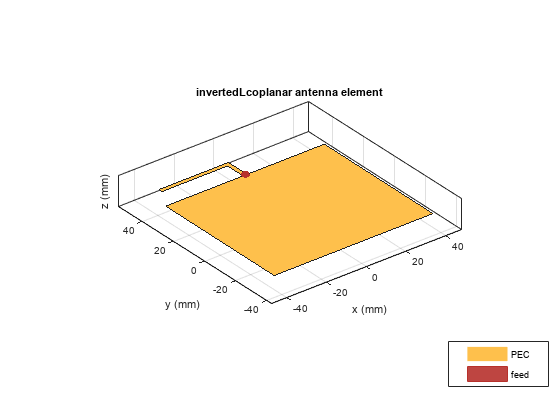
Create a coplanar inverted-L antenna of length 0.050 m, height 0.014 m, ground plane length 0.1 m, and ground plane width 0.1 m.

lco = invertedLcoplanar(Length=50e-3,Height=14e-3,...
    GroundPlaneLength=100e-3,GroundPlaneWidth=100e-3)

lco = 
  invertedLcoplanar with properties:

     RadiatorArmWidth: 0.0020
       FeederArmWidth: 0.0020
               Length: 0.0500
               Height: 0.0140
    GroundPlaneLength: 0.1000
     GroundPlaneWidth: 0.1000
           FeedOffset: 0
            Conductor: [1×1 metal]
                 Tilt: 0
             TiltAxis: [1 0 0]
                 Load: [1×1 lumpedElement]

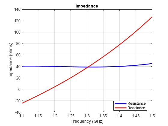
Plot the impedance over 1.1 GHz to 1.5 GHz in steps of 10 MHz.

impedance(lco,1.1e9:10e6:1.5e9);

References

[1] Balanis, C. A. Antenna Theory. Analysis and Design. 3rd Ed. Hoboken, NJ: John Wiley & Sons, 2005.

[2] Stutzman, W. L. and Gary A. Thiele. Antenna Theory and Design. 3rd Ed. River Street, NJ: John Wiley & Sons, 2013.

Version History

Introduced in R2016b