biconeStrip

Create stripped biconical antenna

Since R2020b

Description

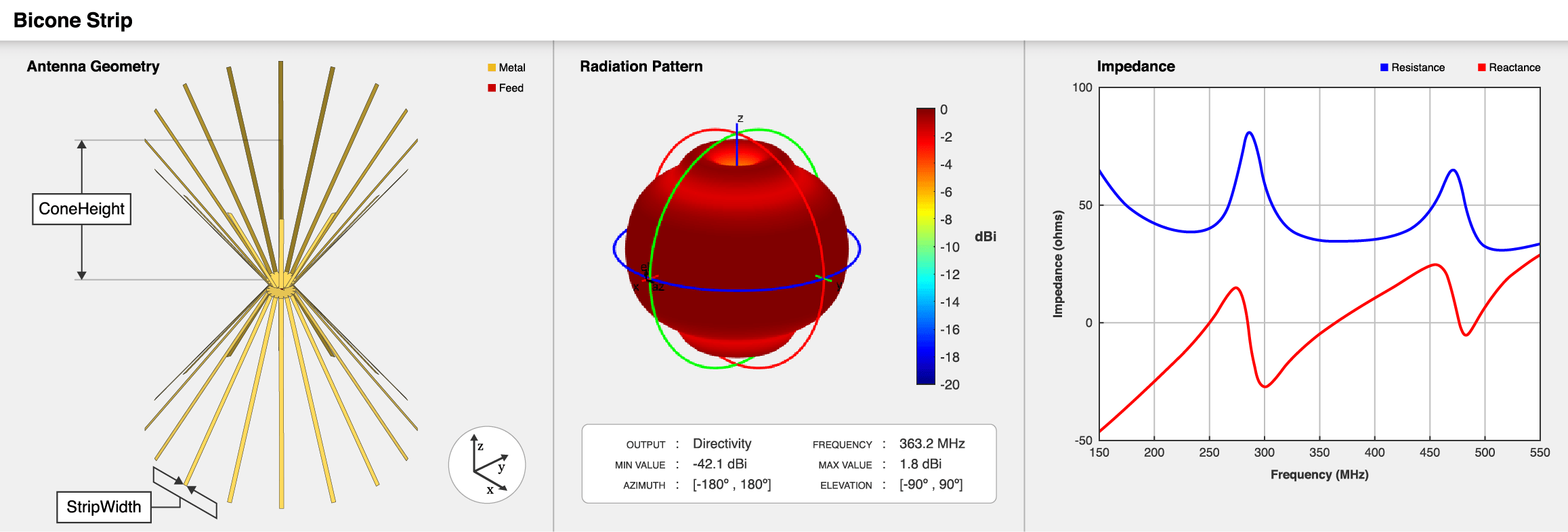
The default biconeStrip object creates a stripped biconical antenna resonating around 363.2 MHz. The stripped biconical antenna is an approximation of a solid biconical antenna, where strips are used to approximate the two cones. The strip configuration makes these antennas lightweight and reduces wind loading. These antennas are more suitable for use at low frequencies. Stripped biconical antennas are popular for their wide-impedance bandwidth and omnidirectional radiation coverage. These antennas are used in applications like emission testing, field monitoring, and chamber characterization.

There are two types of stripped biconical antennas, open-ended and phantom bicones. Specify the HatHeight property to create a phantom stripped biconical antenna.

Creation

Syntax

b = biconeStrip

b = biconeStrip(Name=Value)

Description

b = biconeStrip creates a stripped biconical antenna with default property values. The default dimensions are chosen for an operating frequency of around 363.2 MHz.

b = biconeStrip(Name=Value) sets properties using one or more name-value arguments. Name is the property name and Value is the corresponding value. You can specify several name-value arguments in any order as Name1=Value1,...,NameN=ValueN. Properties that you do not specify, retain their default values.

For example, b = biconeStrip(NumStrips=8) creates a biconical antenna with eight strips and default values for other properties.

Properties

NumStrips — Number of strips to form cones

16 (default) | scalar in the range [6,64]

Number of strips to form the two cones of the stripped biconical antenna, specified a scalar integer in the range [6,64].

Example: 8

Data Types: double

StripWidth — Width of strip

18e-3 (default) | positive scalar

Width of each strip, specified as positive scalar in meters.

Example: 0.02

Data Types: double

HatHeight — Vertical height of hats

0 (default) | positive scalar | two-element vector

Vertical height of the two hats, specified as one of the following options:

• 0 — This creates open-ended stripped biconical antenna.

• Positive scalar in meters — This creates two cone hats of same height.

• Two-element vector with each element unit in meters — This creates two cone hats of different heights. In the two-element vector, the first element specifies the hat height of the top cone, and the second element specifies the hat height of the bottom cone.

Example: 0.045

Data Types: double

ConeHeight — Vertical height of cones

665e-3 (default) | positive scalar | two-element vector

Vertical height of the two cones, specified as one of the following options:

• Positive scalar in meters: This creates two cones of same height.

• Two-element vector with each element unit in meters: This creates two cones of different heights. In the two-element vector, the first element specifies the height of the top cone, and the second element specifies the height of the bottom cone.

Example: 0.5

Data Types: double

NarrowRadius — Radius of apex

70e-3 (default) | positive scalar | two-element vector

Radius at the apex of the cones, specified as one of the following options:

• Positive scalar in meters: This creates two cones with the same narrow radius.

• Two-element vector with each element unit in meters: This creates two cones with different narrow radii. In the two-element vector, the first element specifies the narrow radius of the top cone, and the second element specifies the narrow radius of the bottom cone.

Example: 0.04

Data Types: double

BroadRadius — Radius at broad opening of cone

647e-3 (default) | positive scalar | two-element vector

Radius at the broad opening of the cones, specified as one of the following options:

• Positive scalar in meters: This creates two cones with the same broad radius.

• Two-element vector with each element unit in meters: This creates two cones with different broad radii. In the two-element vector, the first element specifies the broad radius of the top cone, and the second element specifies the broad radius of the bottom cone.

Example: 0.7

Data Types: double

FeedHeight — Height of feed

45e-3 (default) | positive scalar

Height of the feed spanning the gap between the two cones, specified as positive scalar in meters.

Example: 0.04

Data Types: double

FeedWidth — Width of antenna feed

40e-3 (default) | positive scalar

Width of the antenna feed, specified as a positive scalar in meters.

Example: 0.03

Data Types: double

Conductor — Type of metal

metal("PEC") (default) | metal object

Type of the metal used as a conductor, specified as a metal object. You can choose any metal from the MetalCatalog or specify a metal of your choice. For more information on metal conductor meshing, see Meshing.

Example: metal("Copper")

Tilt — Tilt angle of antenna

0 (default) | scalar | vector

Tilt angle of the antenna in degrees, specified as a scalar or vector. For more information, see Rotate Antennas and Arrays.

Example: 90

Example: Tilt=[90 90],TiltAxis=[0 1 0;0 1 1] tilts the antenna at 90 degrees about the two axes defined by the vectors.

Data Types: double

TiltAxis — Tilt axis of antenna

[1 0 0] (default) | three-element vector | 2-by-3 matrix | "X" | "Y" | "Z"

Tilt axis of the antenna, specified as one of these values:

• Three-element vector of Cartesian coordinates in meters. In this case, each coordinate in the vector starts at the origin and lies along the specified points on the x-, y-, and z-axes.

• Two points in space, specified as a 2-by-3 matrix corresponding to two three-element vectors of Cartesian coordinates. In this case, the antenna rotates around the line joining the two points.

• "x", "y", or "z" to describe a rotation about the x-, y-, or z-axis, respectively.

For more information, see Rotate Antennas and Arrays.

Example: [0 1 0]

Example: [0 0 0;0 1 0]

Example: "Z"

Data Types: double | string

Load — Lumped elements

[1x1 lumpedElement] (default) | lumpedElement object

Lumped elements added to the antenna feed, specified as a lumpedElement object. You can add a load anywhere on the surface of the antenna. By default, the load is at the feed.

Example: Load=lumpedElement(Impedance=75)

Example: antenna.Load = lumpedElement(Impedance=75)

Object Functions

axialRatio	Calculate and plot axial ratio of antenna or array
bandwidth	Calculate and plot absolute bandwidth of antenna or array
beamwidth	Beamwidth of antenna
charge	Charge distribution on antenna or array surface
coneangle2size	Calculates equivalent cone height, broad radius, and narrow radius
current	Current distribution on antenna or array surface
design	Design prototype antenna or arrays for resonance around specified frequency or create AI-based antenna from antenna catalog objects
efficiency	Calculate and plot radiation efficiency of antenna or array
EHfields	Electric and magnetic fields of antennas or embedded electric and magnetic fields of antenna element in arrays
feedCurrent	Calculate current at feed for antenna or array
impedance	Calculate and plot input impedance of antenna or scan impedance of array
info	Display information about antenna, array, or platform
memoryEstimate	Estimate memory required to solve antenna or array mesh
mesh	Mesh properties of metal, dielectric antenna, or array structure
meshconfig	Change meshing mode of antenna, array, custom antenna, custom array, or custom geometry
msiwrite	Write antenna or array analysis data to MSI planet file
optimize	Optimize antenna or array using SADEA optimizer
pattern	Plot radiation pattern and phase of antenna or array or embedded pattern of antenna element in array
patternAzimuth	Azimuth plane radiation pattern of antenna or array
patternElevation	Elevation plane radiation pattern of antenna or array
peakRadiation	Calculate and mark maximum radiation points of antenna or array on radiation pattern
rcs	Calculate and plot monostatic and bistatic radar cross section (RCS) of platform, antenna, or array
resonantFrequency	Calculate and plot resonant frequency of antenna
returnLoss	Calculate and plot return loss of antenna or scan return loss of array
show	Display antenna, array structures, shapes, or platform
sparameters	Calculate S-parameters for antenna or array
stlwrite	Write mesh information to STL file
vswr	Calculate and plot voltage standing wave ratio (VSWR) of antenna or array element

Examples

Create Open-ended Strip Bicone Antenna

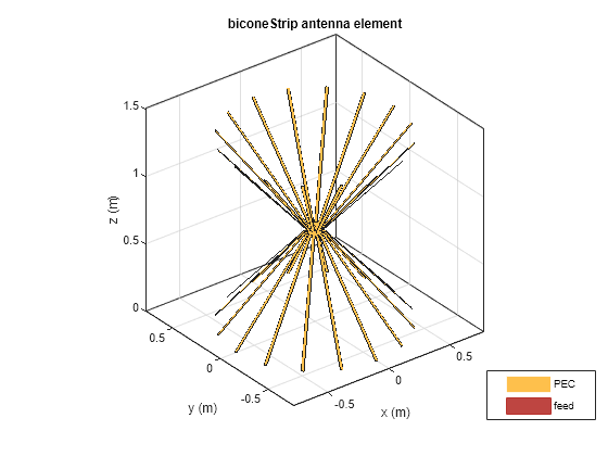
Create a strip bicone antenna with default properties.

ant = biconeStrip

ant = 
  biconeStrip with properties:

       NumStrips: 16
      StripWidth: 0.0180
       HatHeight: 0
      ConeHeight: 0.6650
    NarrowRadius: 0.0700
     BroadRadius: 0.6470
      FeedHeight: 0.0450
       FeedWidth: 0.0400
       Conductor: [1x1 metal]
            Tilt: 0
        TiltAxis: [1 0 0]
            Load: [1x1 lumpedElement]

View the antenna using the show function.

show(ant);

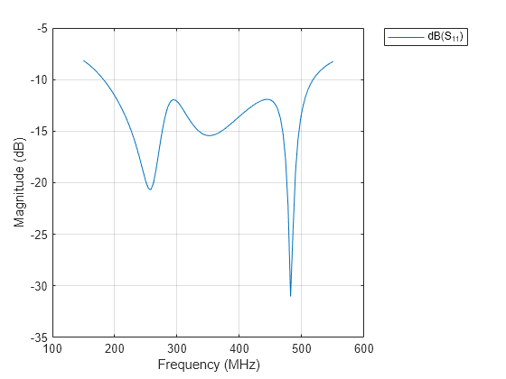
Plot the S-parameters of the antenna over the frequency span of 150-550 MHz.

s = sparameters(ant,linspace(150e6,550e6,101));
rfplot(s)

Create Strip Bicone Antenna with Hat

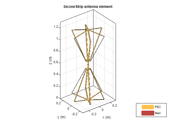
Create a strip bicone antenna with hat.

ant = biconeStrip(NumStrips=6, StripWidth=12e-3, HatHeight=53e-3,...
     ConeHeight=465e-3, NarrowRadius=40e-3, BroadRadius=257e-3,...
     FeedHeight=144e-3, FeedWidth=25e-3);

View the antenna using the show function.

show(ant)

Calculate antenna impedance over the frequency span of 10-300 MHz.

impedance(ant,10e6:10e6:300e6)

More About

Parametric Analysis Guidelines

To understand how the properties of the biconeStrip antenna object influence the antenna design, use the following parametric analysis guidelines.

• To increase the operating frequency, decrease the dimensions of the biconeStrip antenna.

• To increase the impedance bandwidth, use the NumStrips property to increase the number of strips in the biconeStrip antenna object.

• To improve average input impedance, decrease the narrow radii and feed height of the antenna using the NarrowRadius and the FeedHeight properties.

References

[1] Brian A. Austin, Andre P. C. Fourie "Characteristics of the Wire Biconical Antenna Used for EMC Measurements", IEEE Transaction on Electromagnetic Compatibility, vol. 33, no. 3, August 1991.

Version History

Introduced in R2020b