dipoleCylindrical
Create cylindrical dipole antenna
Description
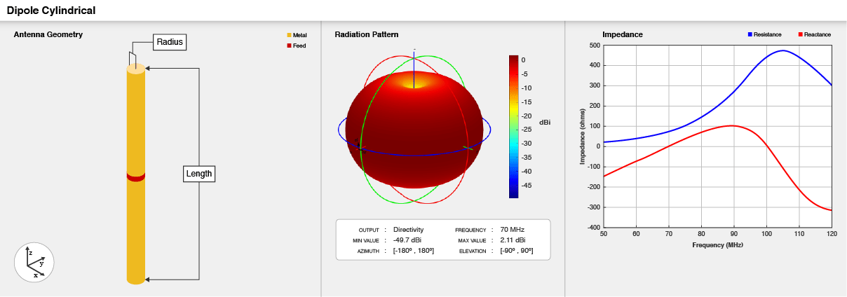
The dipoleCylindrical object creates a center-fed cylindrical
dipole antenna resonating around 70 MHz. The length of the cylindrical dipole corresponds to
half of the wavelength at the operating frequency. These antennas are used in wireless
communication applications requiring thicker dipoles due to their simple
design.
Creation
Description
ant = dipoleCylindrical
ant = dipoleCylindrical(PropertyName=Value)PropertyName is the property
name and Value is the corresponding value. You can specify several
name-value arguments in any order as
PropertyName1=Value1,...,PropertyNameN=ValueN. Properties that you
do not specify, retain their default values.
For example, ant = dipoleCylindrical(Radius=0.04) creates a
cylindrical dipole antenna with radius of 0.04 meters.
Properties
Object Functions
axialRatio | Calculate and plot axial ratio of antenna or array |
bandwidth | Calculate and plot absolute bandwidth of antenna or array |
beamwidth | Beamwidth of antenna |
charge | Charge distribution on antenna or array surface |
current | Current distribution on antenna or array surface |
cylinder2strip | Cylinder equivalent width approximation |
design | Create antenna, array, or AI-based antenna resonating at specified frequency |
efficiency | Calculate and plot radiation efficiency of antenna or array |
EHfields | Electric and magnetic fields of antennas or embedded electric and magnetic fields of antenna element in arrays |
feedCurrent | Calculate current at feed for antenna or array |
impedance | Calculate and plot input impedance of antenna or scan impedance of array |
info | Display information about antenna, array, or platform |
memoryEstimate | Estimate memory required to solve antenna or array mesh |
mesh | Generate and view mesh for antennas, arrays, and custom shapes |
meshconfig | Change meshing mode of antenna, array, custom antenna, custom array, or custom geometry |
msiwrite | Write antenna or array analysis data to MSI planet file |
optimize | Optimize antenna and array catalog elements using SADEA or TR-SADEA algorithm |
pattern | Plot radiation pattern of antenna, array, or embedded element of array |
patternAzimuth | Azimuth plane radiation pattern of antenna or array |
patternElevation | Elevation plane radiation pattern of antenna or array |
peakRadiation | Calculate and mark maximum radiation points of antenna or array on radiation pattern |
rcs | Calculate and plot monostatic and bistatic radar cross section (RCS) of platform, antenna, or array |
resonantFrequency | Calculate and plot resonant frequency of antenna |
returnLoss | Calculate and plot return loss of antenna or scan return loss of array |
show | Display antenna, array, AI-based antenna, platform, or shape |
sparameters | Calculate S-parameters for antenna or array |
stlwrite | Write mesh information to STL file |
strip2cylinder | Calculate equivalent radius approximation for strip |
vswr | Calculate and plot voltage standing wave ratio (VSWR) of antenna or array element |
Examples
Create a cylindrical dipole antenna with default properties.
ant = dipoleCylindrical
ant =
  dipoleCylindrical with properties:

        Length: 2
        Radius: 0.0250
    FeedOffset: 0
     ClosedEnd: 0
     Conductor: [1×1 metal]
          Tilt: 0
      TiltAxis: [1 0 0]
          Load: [1×1 lumpedElement]
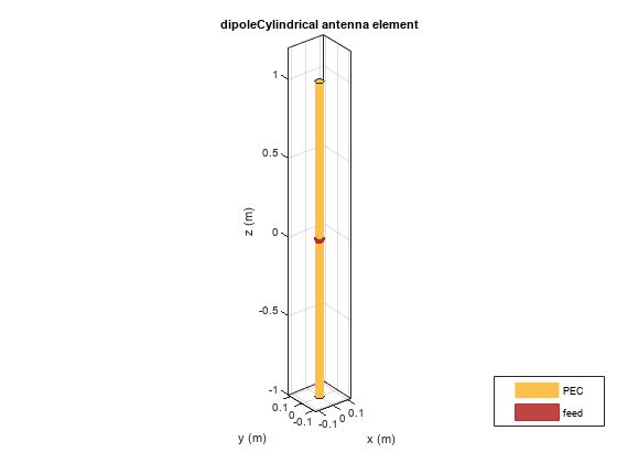
View the antenna using the show function.
show(ant)
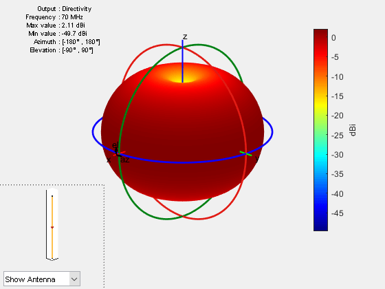
Plot the radiation pattern of the cylindrical dipole antenna at a frequency of 70 MHz.
pattern(ant,70e6)
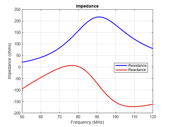
Create a center-fed cylindrical dipole with a length of 2 m and a radius of 0.06 m.
ant = dipoleCylindrical(Length=2, Radius=0.06)
ant =
  dipoleCylindrical with properties:

        Length: 2
        Radius: 0.0600
    FeedOffset: 0
     ClosedEnd: 0
     Conductor: [1×1 metal]
          Tilt: 0
      TiltAxis: [1 0 0]
          Load: [1×1 lumpedElement]
Plot the impedance over a frequency range of 50 MHz to 120 MHz.
impedance(ant,linspace(50e6,120e6,51))
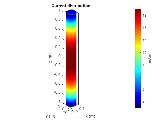
Create cylindrical dipole antennas with an open-ended top and a close-ended top, respectively.
antOpenEnded = dipoleCylindrical(Radius=0.1);
antClosedEnded = dipoleCylindrical(Radius=0.1, ClosedEnd=1);
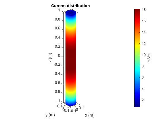
Calculate and plot the current distribution for the cylindrical dipole antennas at frequency of 70 MHz.
iOpenEnded = current(antOpenEnded,70e6)
iOpenEnded = 3×400 complex

  -0.0000 - 0.0002i  -0.0000 - 0.0005i  -0.0000 - 0.0007i  -0.0000 - 0.0005i  -0.0000 - 0.0002i   0.0000 + 0.0002i   0.0000 + 0.0005i   0.0000 + 0.0007i   0.0000 + 0.0005i   0.0000 + 0.0002i   0.0000 + 0.0003i   0.0000 + 0.0007i   0.0000 + 0.0009i   0.0000 + 0.0007i   0.0000 + 0.0003i  -0.0000 - 0.0003i  -0.0000 - 0.0007i  -0.0000 - 0.0009i  -0.0000 - 0.0007i  -0.0000 - 0.0003i  -0.0000 - 0.0001i  -0.0000 - 0.0002i  -0.0000 - 0.0002i  -0.0000 - 0.0002i  -0.0000 - 0.0001i   0.0000 + 0.0001i   0.0000 + 0.0002i   0.0000 + 0.0002i   0.0000 + 0.0002i   0.0000 + 0.0001i   0.0000 + 0.0000i   0.0000 + 0.0001i   0.0001 + 0.0001i   0.0000 + 0.0001i   0.0000 + 0.0000i  -0.0000 - 0.0000i  -0.0000 - 0.0001i  -0.0001 - 0.0001i  -0.0000 - 0.0001i  -0.0000 - 0.0000i  -0.0000 - 0.0000i  -0.0001 - 0.0001i  -0.0001 - 0.0001i  -0.0001 - 0.0001i  -0.0000 - 0.0000i   0.0000 + 0.0000i   0.0001 + 0.0001i   0.0001 + 0.0001i   0.0001 + 0.0001i   0.0000 + 0.0000i
   0.0000 + 0.0006i   0.0000 + 0.0004i   0.0000 + 0.0000i  -0.0000 - 0.0004i  -0.0000 - 0.0006i  -0.0000 - 0.0006i  -0.0000 - 0.0004i   0.0000 + 0.0000i   0.0000 + 0.0004i   0.0000 + 0.0006i  -0.0000 - 0.0008i  -0.0000 - 0.0005i   0.0000 + 0.0000i   0.0000 + 0.0005i   0.0000 + 0.0008i   0.0000 + 0.0008i   0.0000 + 0.0005i   0.0000 + 0.0000i  -0.0000 - 0.0005i  -0.0000 - 0.0008i   0.0000 + 0.0002i   0.0000 + 0.0001i   0.0000 + 0.0000i  -0.0000 - 0.0001i  -0.0000 - 0.0002i  -0.0000 - 0.0002i  -0.0000 - 0.0001i   0.0000 + 0.0000i   0.0000 + 0.0001i   0.0000 + 0.0002i  -0.0001 - 0.0001i  -0.0000 - 0.0001i   0.0000 + 0.0000i   0.0000 + 0.0001i   0.0001 + 0.0001i   0.0001 + 0.0001i   0.0000 + 0.0001i   0.0000 + 0.0000i  -0.0000 - 0.0001i  -0.0001 - 0.0001i   0.0001 + 0.0001i   0.0000 + 0.0000i   0.0000 + 0.0000i  -0.0000 - 0.0000i  -0.0001 - 0.0001i  -0.0001 - 0.0001i  -0.0000 - 0.0000i   0.0000 + 0.0000i   0.0000 + 0.0000i   0.0001 + 0.0001i
  -0.0191 - 0.0016i  -0.0191 - 0.0016i  -0.0191 - 0.0016i  -0.0191 - 0.0016i  -0.0191 - 0.0016i  -0.0191 - 0.0016i  -0.0191 - 0.0016i  -0.0191 - 0.0016i  -0.0191 - 0.0016i  -0.0191 - 0.0016i  -0.0190 + 0.0033i  -0.0190 + 0.0033i  -0.0190 + 0.0033i  -0.0190 + 0.0033i  -0.0190 + 0.0033i  -0.0190 + 0.0033i  -0.0190 + 0.0033i  -0.0190 + 0.0033i  -0.0190 + 0.0033i  -0.0190 + 0.0033i  -0.0189 + 0.0036i  -0.0189 + 0.0036i  -0.0189 + 0.0036i  -0.0189 + 0.0036i  -0.0189 + 0.0036i  -0.0189 + 0.0036i  -0.0189 + 0.0036i  -0.0189 + 0.0036i  -0.0189 + 0.0036i  -0.0189 + 0.0036i  -0.0185 + 0.0046i  -0.0185 + 0.0046i  -0.0185 + 0.0046i  -0.0185 + 0.0046i  -0.0185 + 0.0046i  -0.0185 + 0.0046i  -0.0185 + 0.0046i  -0.0185 + 0.0046i  -0.0185 + 0.0046i  -0.0185 + 0.0046i  -0.0183 + 0.0049i  -0.0183 + 0.0049i  -0.0183 + 0.0049i  -0.0183 + 0.0049i  -0.0183 + 0.0049i  -0.0183 + 0.0049i  -0.0183 + 0.0049i  -0.0183 + 0.0049i  -0.0183 + 0.0049i  -0.0183 + 0.0049i
current(antOpenEnded,70e6)
iClosedEnded = current(antClosedEnded,70e6)
iClosedEnded = 3×428 complex

  -0.0000 - 0.0002i  -0.0000 - 0.0005i  -0.0000 - 0.0007i  -0.0000 - 0.0005i  -0.0000 - 0.0002i   0.0000 + 0.0002i   0.0000 + 0.0005i   0.0000 + 0.0007i   0.0000 + 0.0005i   0.0000 + 0.0002i   0.0000 + 0.0003i   0.0000 + 0.0007i   0.0000 + 0.0008i   0.0000 + 0.0007i   0.0000 + 0.0003i  -0.0000 - 0.0003i  -0.0000 - 0.0007i  -0.0000 - 0.0008i  -0.0000 - 0.0007i  -0.0000 - 0.0003i  -0.0000 - 0.0001i  -0.0000 - 0.0002i  -0.0000 - 0.0002i  -0.0000 - 0.0002i  -0.0000 - 0.0001i   0.0000 + 0.0001i   0.0000 + 0.0002i   0.0000 + 0.0002i   0.0000 + 0.0002i   0.0000 + 0.0001i   0.0000 + 0.0000i   0.0000 + 0.0001i   0.0001 + 0.0001i   0.0000 + 0.0001i   0.0000 + 0.0000i  -0.0000 - 0.0000i  -0.0000 - 0.0001i  -0.0001 - 0.0001i  -0.0000 - 0.0001i  -0.0000 - 0.0000i  -0.0000 - 0.0000i  -0.0001 - 0.0001i  -0.0001 - 0.0001i  -0.0001 - 0.0001i  -0.0000 - 0.0000i   0.0000 + 0.0000i   0.0001 + 0.0001i   0.0001 + 0.0001i   0.0001 + 0.0001i   0.0000 + 0.0000i
   0.0000 + 0.0006i   0.0000 + 0.0004i   0.0000 + 0.0000i  -0.0000 - 0.0004i  -0.0000 - 0.0006i  -0.0000 - 0.0006i  -0.0000 - 0.0004i   0.0000 + 0.0000i   0.0000 + 0.0004i   0.0000 + 0.0006i  -0.0000 - 0.0008i  -0.0000 - 0.0005i   0.0000 + 0.0000i   0.0000 + 0.0005i   0.0000 + 0.0008i   0.0000 + 0.0008i   0.0000 + 0.0005i   0.0000 + 0.0000i  -0.0000 - 0.0005i  -0.0000 - 0.0008i   0.0000 + 0.0002i   0.0000 + 0.0001i   0.0000 + 0.0000i  -0.0000 - 0.0001i  -0.0000 - 0.0002i  -0.0000 - 0.0002i  -0.0000 - 0.0001i   0.0000 + 0.0000i   0.0000 + 0.0001i   0.0000 + 0.0002i  -0.0001 - 0.0001i  -0.0000 - 0.0001i   0.0000 + 0.0000i   0.0000 + 0.0001i   0.0001 + 0.0001i   0.0001 + 0.0001i   0.0000 + 0.0001i   0.0000 + 0.0000i  -0.0000 - 0.0001i  -0.0001 - 0.0001i   0.0001 + 0.0001i   0.0000 + 0.0000i   0.0000 + 0.0000i  -0.0000 - 0.0000i  -0.0001 - 0.0001i  -0.0001 - 0.0001i  -0.0000 - 0.0000i   0.0000 + 0.0000i   0.0000 + 0.0000i   0.0001 + 0.0001i
  -0.0180 - 0.0011i  -0.0180 - 0.0011i  -0.0180 - 0.0010i  -0.0180 - 0.0011i  -0.0180 - 0.0010i  -0.0180 - 0.0010i  -0.0180 - 0.0011i  -0.0180 - 0.0010i  -0.0180 - 0.0011i  -0.0180 - 0.0010i  -0.0179 + 0.0038i  -0.0179 + 0.0038i  -0.0179 + 0.0038i  -0.0179 + 0.0038i  -0.0179 + 0.0038i  -0.0179 + 0.0038i  -0.0179 + 0.0038i  -0.0179 + 0.0038i  -0.0179 + 0.0038i  -0.0179 + 0.0038i  -0.0178 + 0.0041i  -0.0178 + 0.0041i  -0.0178 + 0.0041i  -0.0178 + 0.0041i  -0.0178 + 0.0041i  -0.0178 + 0.0041i  -0.0178 + 0.0041i  -0.0178 + 0.0041i  -0.0178 + 0.0041i  -0.0178 + 0.0041i  -0.0175 + 0.0052i  -0.0175 + 0.0052i  -0.0175 + 0.0052i  -0.0175 + 0.0052i  -0.0175 + 0.0052i  -0.0175 + 0.0052i  -0.0175 + 0.0052i  -0.0175 + 0.0052i  -0.0175 + 0.0052i  -0.0175 + 0.0052i  -0.0173 + 0.0055i  -0.0173 + 0.0055i  -0.0173 + 0.0055i  -0.0173 + 0.0055i  -0.0173 + 0.0055i  -0.0173 + 0.0055i  -0.0173 + 0.0055i  -0.0173 + 0.0055i  -0.0173 + 0.0055i  -0.0173 + 0.0055i
current(antClosedEnded,70e6)
More About
References
[1] King Ronald W.P. Characteristics of Cylindrical Dipoles and Monopoles. Boston, MA: Springer, 1971.
Version History
Introduced in R2021a