dipoleHelix
Create regular or AI-based helical dipole antenna
Description
The default dipoleHelix object is a center-fed helical dipole
antenna resonating around 3.16 GHz. You can move the feed along the antenna length using
the feed offset property. Helical dipoles are used in satellite communications and
wireless power transfers.
The width of the strip is related to the diameter of an equivalent cylinder by this equation
where:
w is the width of the strip.
d is the diameter of an equivalent cylinder.
r is the radius of an equivalent cylinder.
For a given cylinder radius, use the cylinder2strip utility function to calculate the equivalent width. The
default helical dipole antenna is center-fed. Commonly, helical dipole antennas are used
in axial mode. In this mode, the helical dipole circumference is comparable to the
operating wavelength, and has maximum directivity along its axis. In normal mode, the
helical dipole radius is small compared to the operating wavelength. In this mode, the
helical dipole radiates broadside, that is, in the plane perpendicular to its axis. The
basic equation for the helical dipole antenna is:
where:
r is the radius of the helical dipole.
θ is the winding angle.
S is the spacing between turns.
For a given pitch angle in degrees, use the helixpitch2spacing utility function to calculate the spacing between the
turns in meters.
You can perform full-wave EM solver based analysis on the regular
dipoleHelix antenna or you can create a
dipoleHelix type AIAntenna and explore the design
space to tune the antenna for your application using AI-based analysis.
Creation
Description
dh = dipoleHelix
dh = dipoleHelix(PropertyName=Value)PropertyName is the property name
and Value is the corresponding value. You can specify
several name-value arguments in any order as
PropertyName1=Value1,...,PropertyNameN=ValueN.
Properties that you do not specify, retain their default values.
For example, dh = dipoleHelix(Radius=0.02) creates a
helical dipole antenna with a turns radius of 0.02 m and default values for
other properties.
You can also create a regular
dipoleHelixantenna resonating at a desired frequency using thedesignfunction. For example, to create a regulardipoleHelixantenna resonating at 2 GHz, use the following syntax:To analyze this antenna use object functions of the>> design(dipoleHelix,2e9)
dipoleHelix. Use this workflow to design, tune, and analyze adipoleHelixantenna using conventional full-wave solvers.You can create an AI-based
dipoleHelixantenna resonating at a desired frequency using thedesignfunction. Using AI-based antenna models over conventional full-wave solvers significantly reduces the simulation time required to fine-tune the antenna to meet your design goals. Set theForAIargument in thedesignfunction totrueto create adipoleHelixtypeAIAntennaobject. To use this feature, you need license to the Statistics and Machine Learning Toolbox™ in addition to the Antenna Toolbox™. For example, to create an AI-baseddipoleHelixantenna resonating at 2 GHz, use the following syntax:The AI-based>> design(dipoleHelix,2e9,ForAI=true)
dipoleHelixantenna retains the Radius, Width, and Spacing properties of the regulardipoleHelixantenna as tunable properties. Rest of the properties of the regulardipoleHelixantenna are converted into read-only properties in its AI-based version. To find the upper and lower bounds of the tunable properties, use thetunableRangesfunction.To analyze this antenna use object functions of the
AIAntenna. Use this workflow to design, tune, and analyze adipoleHelixantenna using its AI-based model. To create a regulardipoleHelixantenna from this AI-based antenna, use theexportAntennafunction.
Properties
Object Functions
axialRatio | Calculate and plot axial ratio of antenna or array |
bandwidth | Calculate and plot absolute bandwidth of antenna or array |
beamwidth | Beamwidth of antenna |
charge | Charge distribution on antenna or array surface |
current | Current distribution on antenna or array surface |
design | Create antenna, array, or AI-based antenna resonating at specified frequency |
efficiency | Calculate and plot radiation efficiency of antenna or array |
EHfields | Electric and magnetic fields of antennas or embedded electric and magnetic fields of antenna element in arrays |
feedCurrent | Calculate current at feed for antenna or array |
impedance | Calculate and plot input impedance of antenna or scan impedance of array |
info | Display information about antenna, array, or platform |
memoryEstimate | Estimate memory required to solve antenna or array mesh |
mesh | Generate and view mesh for antennas, arrays, and custom shapes |
meshconfig | Change meshing mode of antenna, array, custom antenna, custom array, or custom geometry |
msiwrite | Write antenna or array analysis data to MSI planet file |
optimize | Optimize antenna and array catalog elements using SADEA or TR-SADEA algorithm |
pattern | Plot radiation pattern of antenna, array, or embedded element of array |
patternAzimuth | Azimuth plane radiation pattern of antenna or array |
patternElevation | Elevation plane radiation pattern of antenna or array |
peakRadiation | Calculate and mark maximum radiation points of antenna or array on radiation pattern |
rcs | Calculate and plot monostatic and bistatic radar cross section (RCS) of platform, antenna, or array |
resonantFrequency | Calculate and plot resonant frequency of antenna |
returnLoss | Calculate and plot return loss of antenna or scan return loss of array |
show | Display antenna, array, AI-based antenna, platform, or shape |
sparameters | Calculate S-parameters for antenna or array |
stlwrite | Write mesh information to STL file |
vswr | Calculate and plot voltage standing wave ratio (VSWR) of antenna or array element |
wireStack | Create single or multi-feed wire antenna |
Examples
Create a default helical dipole antenna and view it.
dh = dipoleHelix
dh =
  dipoleHelix with properties:

              Radius: 0.0220
               Width: 1.0000e-03
               Turns: 3
             Spacing: 0.0350
    WindingDirection: 'CCW'
          FeedOffset: 0
           Substrate: [1×1 dielectric]
           Conductor: [1×1 metal]
                Tilt: 0
            TiltAxis: [1 0 0]
                Load: [1×1 lumpedElement]
show(dh)

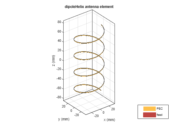
Create a four-turn helical dipole antenna with a turn radius of 28 mm and a strip width of 1.2 mm.
dh = dipoleHelix(Radius=28e-3, Width=1.2e-3, Turns=4);
show(dh)
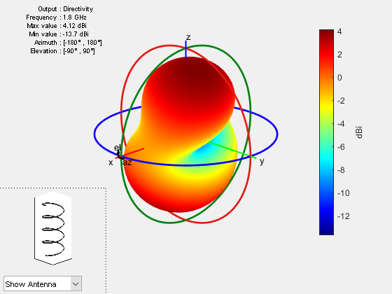
Plot the radiation pattern of the helical dipole at 1.8 GHz.
pattern(dh, 1.8e9);
Create a custom dipole helix antenna with a Teflon dielectric substrate.
d = dielectric('Teflon');
dh = dipoleHelix(Radius=22e-3,Width=1e-3,Turns=3,Spacing=35e-3,FeedOffset=0,Substrate=d)
dh =
dipoleHelix with properties:
Radius: 0.0220
Width: 1.0000e-03
Turns: 3
Spacing: 0.0350
WindingDirection: 'CCW'
FeedOffset: 0
Substrate: [1×1 dielectric]
Conductor: [1×1 metal]
Tilt: 0
TiltAxis: [1 0 0]
Load: [1×1 lumpedElement]
View the dipole helix antenna.
show(dh)

This example shows how to design a helical dipole antenna that resonates at 2 GHz.
Design Helical Dipole
Use the design function to create a helical dipole antenna that resonates at 2 GHz.
dh = design(dipoleHelix,2e9)
dh =
  dipoleHelix with properties:

              Radius: 0.0171
               Width: 0.0016
               Turns: 15
             Spacing: 0.0239
    WindingDirection: 'CW'
          FeedOffset: 0
           Substrate: [1×1 dielectric]
           Conductor: [1×1 metal]
                Tilt: 0
            TiltAxis: [1 0 0]
                Load: [1×1 lumpedElement]
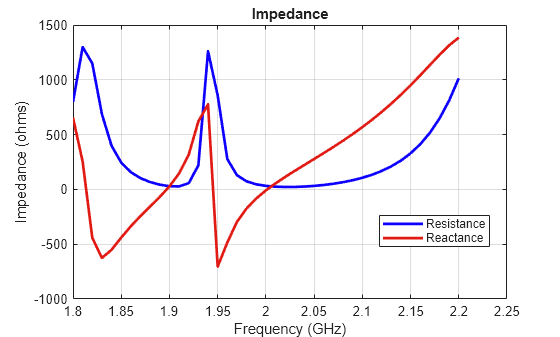
Plot Impedance of Helical Dipole
Use the impedance function to plot the impedance of the helical dipole antenna in 1.8 GHz to 2.2 GHz range.
figure
impedance(dh,1.8e9:10e6:2.2e9)
This example shows how to create an AI-based helical dipole antenna at 2 GHz and calculate its resonant frequency.
pAI = design(dipoleHelix,2e9,ForAI=true)
pAI =
  AIAntenna with properties:

   Antenna Info
               AntennaType: 'dipoleHelix'
    InitialDesignFrequency: 2.0000e+09

   Tunable Parameters
                    Radius: 0.0171
                   Spacing: 0.0239
                     Width: 0.0016

Show read-only properties
showReadOnlyProperties(pAI)
                      Turns: 15
           WindingDirection: 'CW'
                 FeedOffset: 0

              SubstrateName: 'Air'
          SubstrateEpsilonR: 1
       SubstrateLossTangent: 0
         SubstrateThickness: 0.3602
    SubstrateFrequencyModel: 'Constant'

              ConductorName: 'PEC'
      ConductorConductivity: Inf
         ConductorThickness: 0

                       Tilt: 0
                   TiltAxis: [1 0 0]

              LoadImpedance: []
              LoadFrequency: []
               LoadLocation: 'feed'
Vary the helix radius, turns spacing, and width. Calculate its resonant frequency.
pAI.Radius = 0.0146;
pAI.Spacing = 0.021;
pAI.Width = 0.0014;
fR = resonantFrequency(pAI)
fR =
1.9960e+09
Convert the AIAntenna to a regular helical dipole antenna.
dh = exportAntenna(pAI)
dh =
  dipoleHelix with properties:

              Radius: 0.0146
               Width: 0.0014
               Turns: 15
             Spacing: 0.0210
    WindingDirection: 'CW'
          FeedOffset: 0
           Substrate: [1×1 dielectric]
           Conductor: [1×1 metal]
                Tilt: 0
            TiltAxis: [1 0 0]
                Load: [1×1 lumpedElement]
References
[1] Balanis, C. A. Antenna Theory. Analysis and Design. 3rd Ed. Hoboken, NJ: John Wiley & Sons, 2005.
[2] Volakis, John. Antenna Engineering Handbook. 4th Ed. New York: McGraw-Hill, 2007.